I am interested in using an optimization technique called Bayesian optimization in a current research project, so I wanted to take this opportunity to write a couple of blog posts to describe how this algorithm works. Generally speaking, Bayesian optimization is an appropriate tool to use when you are trying to optimize a function that you do not have an analytical expression for (i.e. that is a black-box function) and when it is expensive to evaluate that function [1]. In this post, I will describe in more detail when Bayesian optimization is useful, and how it works from a mathematical standpoint. I may write an accompanying blog post that dives into some of the relevant mathematical tools more deeply, as well. Let’s get started!

Introduction to Bayesian Optimization

As I mentioned in the introduction, Bayesian optimization is a good tool to use when you want to optimize a function \(f(x)\) (which we call the objective function) and it has the following two properties [1]:

• The analytical expression for \(f(x)\) is unknown (it is a black box). In this situation, we cannot use other techniques like finding the optimal solution analytically because we don’t have the expression to work with.

• The cost of finding \(f(x)\) for a given value of \(x\) is very high. This is often true in experimental settings, where \(f(x)\) refers to a physical process that we are studying, or when we are trying to optimize the hyperparameters of a neural network, and each time we choose a set of hyperparameters we have to completely re-train the network. If this was not true, we could use simpler approaches like grid search to find the optimal value of \(x\), because each evaluation of \(f(x)\) would be cheap.

Let’s assume that we find ourselves in a situation where \(f(x)\) meets both of these conditions. In this case, we can use Bayesian optimization to find \(x^{*}\), the globally optimal value of \(x\), while minimizing the number of times that we query \(f(x)\). In other words, our objective is [2]:

\[\max_{x} f(x)\]

The Bayesian part of Bayesian optimization comes from the fact that we will incorporate samples drawn from the objective function into our prediction for the optimal value of \(x\). As we will see in a moment, we will define a prior (i.e. a guess) for \(x^*\) and as we draw samples from the objective function, we will update the prior to define a posterior that includes our samples to give a more accurate guess of what \(x^*\) is. Note that, even though sampling the objective function is expensive, we will have to draw samples during this process, but we will try to minimize the number of samples that we need to draw before we can identify \(x^*\) [1].

I will give an intuitive explanation of how Bayesian optimization works and then present the mathematics in the next section. Bayesian optimization uses two functions to guide the optimization process: a surrogate function and an acquisition function. The surrogate function, \(g(\cdot)\), addresses the problem described above where we have no analytical expression for \(f(x)\) - the surrogate function acts as our best guess of the form of \(f(x)\) given the current information. The acquisition function, \(u(\cdot)\), guides our choice of the next sample of \(x\) to sample from the objective function. The acquisition function must balance exploration and exploitation to find the globally optimal value of \(x\) as quickly as possible. Note that the acquisition function uses the surrogate function as we will see in the next section [1].

Once we have defined the surrogate and acquisition functions, we can use them in an iterative process to optimize the objective function as follows [1]:

1. Iterate for \(t = 1, 2, …, T\) steps for sampled points, \((\mathbf{x}, y)\), that are added to the set \(\mathcal{D}_{1:t-1}\).

2. Select the next point to sample, \(\mathbf{x}_t\), by finding the argmax of the acquisition function, i.e.:

\[\mathbf{x}_t = \text{argmax}_{\mathbf{x}} u(\mathbf{x} | \mathcal{D}_{1:t-1})\]

1. Sample the objective function at this point: \(y_t = f(\mathbf{x}_t)\). Add this sample to the set, \(\mathcal{D}_{1:t} = \{\mathcal{D}_{1:t-1}, (\mathbf{x}_t, y_t)\}\).

2. Update the surrogate function, \(g(\cdot)\) with the newly sampled point \((\mathbf{x}_t, y_t)\).

Now let’s dive into the mathematics of this approach in more detail.

The Math Behind the Surrogate and Acquisition Functions

The surrogate function’s purpose is to represent our best guess of the analytic form of the objective function, \(f(x)\). One commonly used form for the surrogate function is a Gaussian process [1,3]. I will write a separate blog post to describe the mathematics behind Gaussian processes (GPs) because they are really cool and deserve more attention. For the purposes of this discussion, let me just briefly say that GPs represent a collection of functions, and each function has some probability that it is the best fit to the observed data [4]. A GP will represent the process as a joint probability over a set of random variables, where each random variable corresponds to one data point, and the set of points follows a multivariate normal distribution [5]. The benefit of using a Gaussian (or normal) representation is that it has many useful properties that make it easier to update the probability distribution using Bayes’ rule. As I said, GPs are really interesting tools so please look for another post coming soon that dives into their mechanics in much more detail*1.

So our best guess at the objective function is represented by a GP, but what about the acquisition function? There are multiple approaches to writing the acquisition function, including probability of improvement, expected improvement, and Thompson sampling [3]. However, I will just focus on expected improvement (EI) for this post, and we can assume that other approaches will fit into the Bayesian optimization algorithm in a similar fashion.

The EI approach balances exploitation and exploration as it recommends the next query point, \(\mathbf{x}_t\). Specifically, the EI approach will select a query point either because it is bigger than the best value we have seen so far (exploitation) or because that point is in a region of high uncertainty (exploration). The expression for EI can be written as [3]:

\[\mathbf{x}_{t+1} = \text{argmax}_{\mathbf{x}} \mathbb{E} \left( \max \{ g_{t+1}(\mathbf{x}) - f(\mathbf{x}^+), 0 \} | \mathcal{D}_{1:t} \right)\]

Here, we are choosing the next query point, \(\mathbb{x}_{t+1}\) as the value that maximizes the surrogate function, \(g_{t+1}(\mathbf{x})\), compared to the best value that we’ve seen so far, represented by \(f(\mathbf{x}^+)\). This choice is conditioned on all of the data we have to date, \(\mathcal{D}_{1:t}\) [3].

Since we know the specific form of the surrogate function, \(g(\cdot)\), is as a GP, we can write an analytical expression for the equation above as follows [3]:

\[EI(\mathbf{x}) = \begin{cases} (\mu_t(\mathbf{x}) - f(\mathbf{x}^+) - \zeta)\Phi(Z) + \sigma_t(\mathbf{x})\phi(Z) & \text{if $\sigma_t(\mathbf{x}) > 0$} \\ 0 & \text{if $\sigma_t(\mathbf{x}) = 0$} \end{cases}\]

Where \(\mu_t\) and \(\sigma_t\) are the mean and variance of the GP, and \(\Phi(Z)\) and \(\phi(Z)\) are the CDF and PDF of the GP, respectively. The first term represents the exploitation (because it drives the selection of the query point that maximizes the surrogate function) while the second term represents the exploration (because it favors selecting the query point that is in the area of greatest uncertainty, as represented by the variance, \(\sigma_t\)). The parameter \(\zeta\) controls the trade-off between these two terms representing exploration and exploitation [1,3]. Finally, \(Z\) is [1,3]:

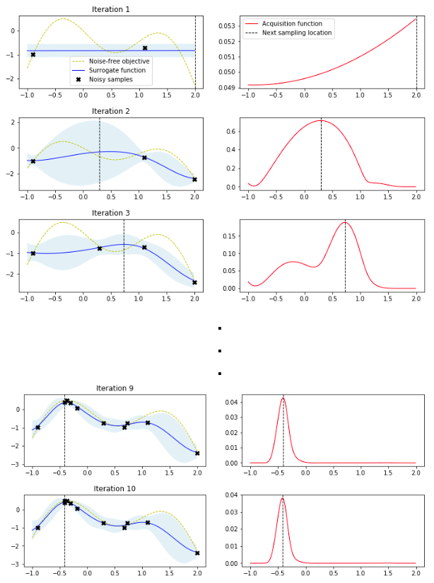
\[Z = \begin{cases} \frac{\mu_t(\mathbf{x}) - f(\mathbf{x}^+) - \zeta}{\sigma_t(\mathbf{x})} & \text{if $\sigma_t(\mathbf{x}) > 0$} \\ 0 & \text{if $\sigma_t(\mathbf{x}) = 0$} \end{cases}\]

This math is everything that is required to implement Bayesian optimization. Krasser presents a beautiful Colab notebook that implements the algorithm from scratch and plots the results in a highly intuitive manner. I recreate part of the key figure below but I would recommend exploring his blog post and accompanying notebook to get a better understanding of how the Bayesian optimization algorithm can unfold on an example system [1].

Figure [1] - Source [1]

Conclusion

In this post we discussed how Bayesian optimization works and when one would want to use it. In a follow-up post, I will dig more deeply into one of the mathematical tools we used in this algorithm, Gaussian processes. Thanks for reading and stay tuned!

Footnotes

*1 Or just read this amazing Distill article by Görtler, et al.

References

[1] Krasser, M. “Bayesian optimization.” 21 Mar 2018. http://krasserm.github.io/2018/03/21/bayesian-optimization/ Visited 4 Jun 2022.

[2] “Bayesian optimization.” Wikipedia. https://en.wikipedia.org/wiki/Bayesian_optimization Visited 4 Jun 2022.

[3] Agnihotri & Batra, “Exploring Bayesian Optimization”, Distill, 2020. https://distill.pub/2020/bayesian-optimization/ Visited 4 Jun 2022.

[4] Görtler, et al., “A Visual Exploration of Gaussian Processes”, Distill, 2019. https://distill.pub/2019/visual-exploration-gaussian-processes/ Visited 4 Jun 2022.

[5] “Gaussian process.” Wikipedia. https://en.wikipedia.org/wiki/Gaussian_process Visited 4 Jun 2022.