In this post we are going to talk about binary search trees, which is a specific type of tree, which itself is a more general data structure. Trees have a lot of uses and variants in computer science, so this post is only going to scratch the surface of what it is possible to do with trees. Laakmann McDowell points out that, because there are so many varieties of trees in computer science, as well as varied terminology, it is important to ask lots of clarification questions with your interviewer if you encounter a tree during a coding interview [1]. In this post, we will discuss some of the basic theory behind trees, the specific properties of binary search trees, and some of the operations you can perform on them. I also have some implementations of trees in Python available here; these implementations draw heavily on tutorials by [2-3].

Basic Components of a (Binary Search) Tree

Generally, all types of tree implementations share some common features, which are all illustrated in Figure 1. The tree will have a root node, which can be identified because it will not have any parent nodes, only zero or more child nodes [1]. Each child node will itself have zero or more children [1]. Unlike a graph, a tree cannot have cycles [1]. The last row of nodes in a tree are typically called leaf nodes, and they can be identified because they will not have any child nodes [1]. Typically the nodes store keys from key-value pairs, and they will also either store the value itself or a pointer to it [4].

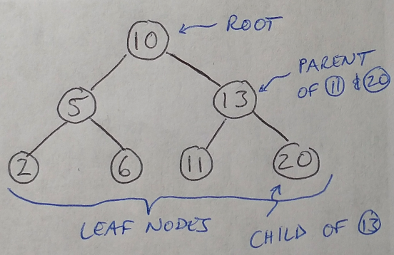
Figure 1

Other details about trees can vary widely, such as how they are ordered, what data types they store, how parent and child nodes can be linked, and so on [1]. Since this post is about binary search trees in particular, their specific characteristics include the fact that every node is limited to having a maximum of 2 child nodes, and that all nodes are ordered according to a specific ordering property [1]. Specifically, all left descendants must be less than or equal to node n*1, and all right descendants must be greater than node n, and this must be true for all nodes n in the tree [1]. This is illustrated in Figure 1, where you can see that all of the nodes in the tree follow this ordering property.

I want to point out that there is also a separate, more general category of trees called binary trees and binary search trees are a subset of this category [1]. Both categories apply the limit of a maximum of two child nodes per parent node, but only binary search trees require that the nodes are sorted in a specific order, where left-hand nodes are smaller than right-hand nodes [1]. Binary search trees can be used, for example, to implement dictionaries [4] (although in Python they are actually implemented with hash tables [5]).

Trees have some other characteristics that we often discuss when working with them. For example, sometimes we say that we are working with balanced or unbalanced trees, and this refers to how the nodes are distributed within the tree structure [1]. They are qualitative descriptions, but in general a balanced tree can be thought of as having enough nodes distributed uniformly across the tree that the find and insert functions can be done in O(log n) time (more on this later) [1].

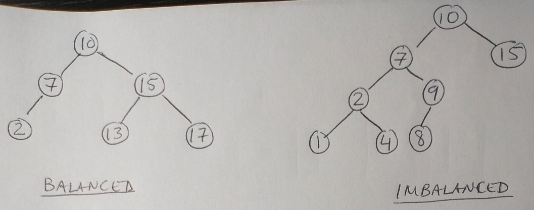
Figure 2

We can also describe a tree as being complete if every level of the tree is completely filled (i.e. every node has 2 children in the case of binary trees) except for, perhaps, the last level (the leafs) [1]. Complete trees are not to be confused with full trees, where every node has either 0 or 2 child nodes [1]. And lastly we can have perfect trees where the trees are both full and complete [1]. This means that all leaf nodes must be at the same level of the tree, and the last level has the maximum number of nodes [1]. Laakmann McDowell warns that perfect trees are rare in interviews, so you should ask your interviewer before assuming that you have one [1].

Now that we have some idea of the structure of a binary search tree, let’s look at some of the operations we can perform on them.

Operations with Binary Search Trees

First we will look at 3 different ways to traverse a tree (i.e. ways to move over all the nodes), then we will look at find, insert and delete operations on nodes in a binary search tree. The 3 traversal methods for trees are [1]:

1. In-order traversal: we visit the left branch, then the current node, then the right branch. When in-order traversal is applied to binary search trees, we will automatically visit all the nodes in ascending order. (In reality “visiting” means that we are printing the contents of the node to the terminal.)

2. Pre-order traversal: first we visit the current node, then we visit the child nodes from left to right. We always visit the root node first.

3. Post-order traversal: contrary to pre-order traversal, we start with visiting the child nodes from left to right, and then visit the current node. The root node is always the last one visited.

The find operation for trees will look for a node of a specific value. In binary search trees, the find operation is quite simple: we start at the root and choose to go to the left child if the value we are looking for is less than the root, and we go right if it is greater than the root [4]. We repeat this process of going left or right until we find the node we are looking for, or we reach the bottom of the tree, in which case that value is not present in the tree [4]. A variant of find, known as findmin, looks for the minimum value in the tree by always choosing the left-hand child at every level.

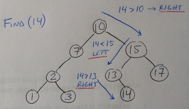
Figure 3

The insert operation simply uses find until the node closest in value to the value to insert is found. We then add a new node at the correct location (left or right of the current node whose value is closest to the value to insert) [4].

The delete operation is slightly more complicated, because there are 3 possible cases when we need to delete a node [4]. The easiest case is that the node to delete is a leaf, in which case we can simply delete it [4].

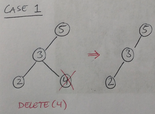
Figure 4

The second possible case is that the node to delete has one child. In this case, we delete the node and move the child up to take its place [4].

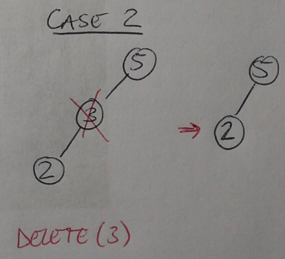
Figure 5

Finally, the third possible case is that the node has two child nodes. Here, we must find the minimum of the right-hand subtree that extends below the node to delete [4]. This value is the next largest value after the node that we need to delete. We move it up to take the place of the deleted node [4].

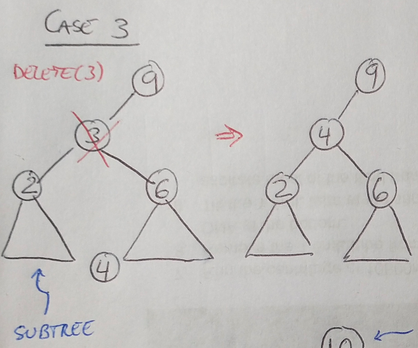
Figure 6

The runtime for find, findmin, as well as insert and delete usually depends on the number of levels in the tree, although this can vary depending on how the tree is implemented - for example, in C++ the runtime will take O(log n) time, but for Perl and Python it takes O(1) time [4]. Let’s take a minute to understand why it might take O(log n) time to complete the find/insert/delete operations for a binary search tree. First, we can define the height of the tree as the number of levels, h, it contains. Then the total number of nodes, n, in the tree, is, at most:

Equation 1

If we want to solve for the height of the tree, then we take the logarithm (base 2) of both sides to say that the height of the tree is log n [6]. Notice that this estimate for the height of the tree assumes that the tree is fairly well balanced, and may become inaccurate if that assumption is incorrect (see below). So if the find operation needs to visit one node in every level of the tree (the same is true for the insert operation), and we assume that visiting itself takes constant time, then the total run time of the find/insert operations is just O(log n) [6]. In other words, the runtime is just dependent on the height of the tree.

This brings us to a discussion about imbalance partitioning in trees. If we have done a poor job of partitioning the nodes in the tree, then one side of the tree will have a lot more nodes than the other. This will add additional levels to the tree, defeating the purpose of having a tree, because the value of the tree is that it makes it possible to find nodes in O(log n) time, not O(n) time, as it does in a sequential search [4]. Depending on the application, it may be necessary to force the binary search tree to remain balanced as we insert and delete nodes [4]. This can be done using B trees or splay trees, and I may try to explain those more in a future post, but for now it’s enough just to know that this problem exists and that there are solutions for it [4].

Footnotes:

*1 Laakmann McDowell recommends asking your interviewer (if you encounter a binary search tree during your coding interview) whether duplicates are allowed in the binary search tree or not [1]. This will be important when you are inserting nodes into the tree.

References:

[1] Laakmann McDowell, G. Cracking the Coding Interview, 6th edition. 2016. CareerCup, LLC.

[2] Leon, K. “Making Data Trees in Python.” The Startup at Medium. 24 Feb 2020. https://medium.com/swlh/making-data-trees-in-python-3a3ceb050cfd Visited 17 Jan 2021.

[3] Gadige, M. “Binary Trees in Python.” Edpresso. https://www.educative.io/edpresso/binary-trees-in-python Visited 17 Jan 2021.

[4] Kingsford, C. and Ma, J. “Splay Trees.” 15-351/15-650/02-613 Algorithms and Advanced Data Structures, Fall 2020.

[5] “How are Python’s Built In Dictionaries Implemented?” Stack Overflow. https://stackoverflow.com/questions/327311/how-are-pythons-built-in-dictionaries-implemented Visited 17 Jan 2021.

[6] Kingsford, C. and Ma, J. “Heaps.” 15-351/15-650/02-613 Algorithms and Advanced Data Structures, Fall 2020.