This post is going to be about understanding Bode plots and how to draw them. The Bode plot is the preferred way of depicting a system’s response in the frequency domain. It is popular among hardware engineers because it allows you to see how your system will behave over a wide range of frequencies and design accordingly. It can be obtained experimentally by providing inputs to the system and measuring the output frequencies (if the system is stable) and it can also be obtained by hand (even if the system is not stable) [1]. The tricky thing about Bode plots is that they will not always tell you if your system is unstable or not. As we will see in an example, it is possible to draw a perfectly normal-looking Bode plot for a system that we know is unstable [2].

A Bode plot is actually comprised of two plots, the magnitude and phase plots. It tells you how an input sine wave of any frequency will be transformed by the system. If you recall my post on linear time-invariant (LTI) systems, you will understand that such systems can scale and add responses together, but they cannot change the frequency of the output response [3]. This is very important: LTI systems DO NOT change the frequency of the output sine wave from the input frequency [3]. LTI systems can change the amplitude of the output sine wave, and they can shift the sine wave in time (i.e. apply a phase shift) but they will never change the output frequency [3]. This is why we can use the frequency as the x-axis for the Bode plot, and then examine how the system will affect the magnitude (i.e. the amplitude of the output relative to the input) and the phase (i.e the time shift of the output relative to the input).

Notice that the Bode plot is logarithmic in both the frequency and magnitude axes (phase is linear). There is an interesting bit of history on why we use decibels to represent the magnitude which I will describe another time [3]. But here it is important to note that I will typically use radians as my unit of frequency, decibels for magnitude and degrees for phase, but it is possible to use other units as well.

As we begin to sketch Bode plots below, you will see that we consistently substitute s = j.omega (j times omega) [1]. But if you remember my post on Fourier and Laplace transforms, s = sigma + j.omega, so why do we ignore sigma? We intentionally separate the forced (steady state) solution from the natural (transient) solution [1]. The sigma portion dictates the transient response of the system, while the j.omega portion dictates the steady state response. Recall Euler’s equation which allows us to convert the exponent of j.omega into a sinusoidal expression, which represents the long-term oscillations of the system [3]. The exponent of sigma only describes how the system will decay over time - this is called the transient response. The Bode plot is useful specifically because it allows us to design for the steady state response of a system over the entire frequency operating range, which is why we focus on the j.omega term.

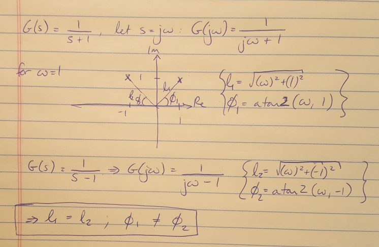
Note that when sketching a Bode plot for a 1st order pole or zero, the math does not care if the pole/zero is in the right or left half plane [2]. The Bode plot is showing the magnitude contributions of that pole and zero which is independent of the location of the pole and zero. However, the phase will be reversed from positive to negative if the pole/zero is in the right half plane [2]. To see that this is true, recall that we can get the magnitude and phase information for a pole/zero from the root locus. If we compare this information for a pole in the right half vs the left half plane, we can see that the magnitude is the same but the angles are separated by 180 degrees. Therefore, you could draw a Bode plot for an unstable system which looks perfectly normal and functional, until you inspect the transfer function and the root locus and see that the system is unstable. I guess the moral of that story is: ALWAYS DRAW A ROOT LOCUS AND A BODE PLOT! We’ll also talk about using Nyquist plots as another tool for checking stability…

Figure 1: Calculating the phase and magnitude for a LHP and RHP pole.

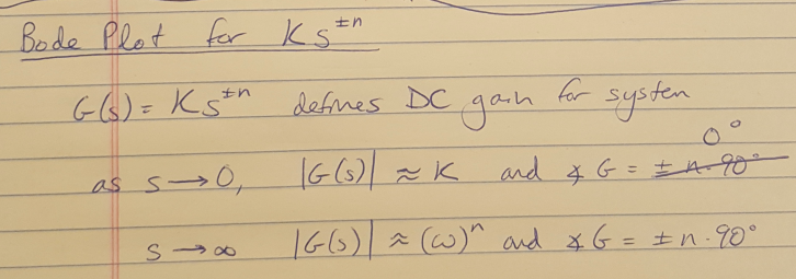
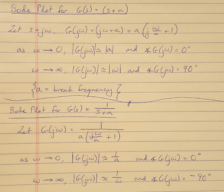
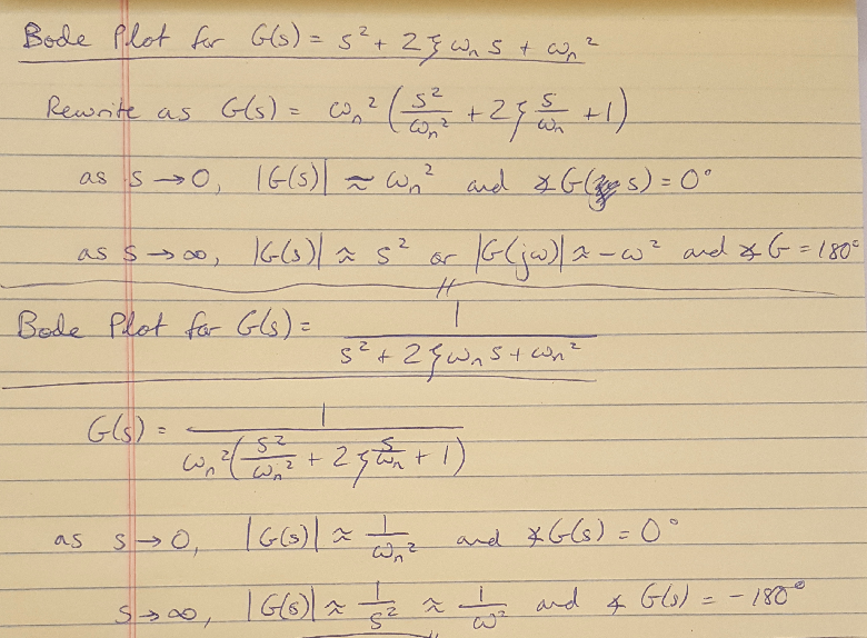
I think that the rules for drawing Bode plots are pretty well documented elsewhere so I have just put my handwritten notes at the bottom of this post for reference. I would recommend visiting Swarthmore’s website for a very detailed explanation of drawing Bode plots if you need a place to practice [4].

Figure 2: Bode plot rules for zero order terms.

Figure 3: Bode plot rules for first order terms.

Figure 4: Bode plot rules for second order terms.

References

[1] Nise, Norman S. Control Systems Engineering, 4th Ed. John Wiley & Sons, Inc. 2004.

[2] Franklin, G., Powell, J.D., Emami-Naeini, A. Feedback Control of Dynamic Systems, 6th ed. Pearson. 2009.

[3] Douglas, Brian. “Control System Lectures - Bode Plots, Introduction.” https://www.youtube.com/watch?v=_eh1conN6YM&list=PLUMWjy5jgHK1NC52DXXrriwihVrYZKqjk&index=9 Visited on 08/14/2019.

[4] Cheever, Erik. “Bode Plots Overview.” https://lpsa.swarthmore.edu/Bode/Bode.html Visited on 08/15/2019.