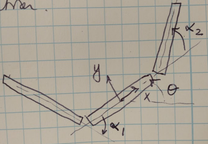
In this post we are going to talk about connection vector fields and connection curvature functions. These are two mathematical tools used to study robot locomotion. I have been using them in my research lately, and I wanted to provide a rigorous explanation of what they are and how to use them. For the purposes of this discussion, we are going to assume that we have a 3 link swimming robot where we know the angle of each link and the orientation and position of the entire robot system. This robot is shown in Figure 1. In this case, the connection vector fields and connection curvature functions can both help us to study how the joint angles impact the system orientation and position. Let’s dive in to see how this works!

Figure 1 - inspired by [1]

The General Reconstruction Equation

We begin by introducing the general reconstruction equation, which is used to map the joint angle velocities, \(\dot{r}\) to the body velocity, \(\xi\), of the robot system [1]:

\[\xi = -\mathbf{A}(r) \dot{r} + \mathbf{\Gamma}(r) p\]

Where \(\mathbf{A}(r)\) is the local connection that maps the joint velocities to body velocity, and \(\mathbf{\Gamma}(r)\) is the momentum distribution function, and \(p\) is the generalized momentum. For the purposes of this discussion, let’s assume that our robot has zero momentum (for example, if it was in a low Reynolds number environment). That cleans up our equation above to a specific form called the kinematic reconstruction equation [1]:

\[\xi = -\mathbf{A}(r) \dot{r}\]

The matrix \(\mathbf{A}(r)\) is going to be the key to studying our robot system in the next sections.

Connection Vector Fields

The problem with expressions for the local connection, \(\mathbf{A}(r)\), is that they can be complicated and difficult to parse by inspection. However, if we plot the local connection, we can learn useful things about our robot system’s locomotion. One way to think about \(\mathbf{A}(r)\) is to understand that each row of the matrix, when dotted with the joint velocities, \(\dot{r}\), produces the velocity of the robot system in the corresponding body velocity component. Mathematically speaking [1]:

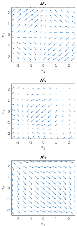
\[\xi_{i} = \mathbf{A}^{i}(r) \cdot \dot{r}\] \[\left[ \matrix{\xi_{x} \cr \xi_y \cr \xi_{\theta}} \right] = \left[ \matrix{A^{x,1}(r) & A^{x,2}(r) \cr A^{y,1}(r) & A^{y,2}(r) \cr A^{\theta,1}(r) & A^{\theta,2}(r)} \right] \cdot \left[ \matrix{\dot{\alpha}_1 \cr \dot{\alpha}_2} \right]\]

Once we compute this dot product, we can plot how each body position coordinate (x, y and \(\theta\)) changes as the joint angles \(\alpha_1\) and \(\alpha_2\) change. This is called the connection vector field, and an example of the connection vector fields for a 3 link microswimmer is shown in Figure 2. If there is a change in the joint angles that follows the arrows (i.e. gradient, or direction of change) of the connection vector field, that means that the corresponding body position is also changing. If, instead, the joint angles of the robot are changing in a way that is orthogonal to the vector field, then that would result in a net zero motion for that corresponding body position [1].

Figure 2 - inspired by [1]

The connection vector fields shown in Figure 2 have some physically relevant information. First of all, if we look at the plot for \(\theta\), we can see that the gradient is generally moving towards \(\mathbf{\alpha} = (+\alpha_1, -\alpha_2)\), suggesting that the entire orientation of the microswimmer prefers to rotate against the direction of rotation of the outer links as compared to the center. Secondly, for the \(\mathbf{A}^x\) plot we can see that the gradient of the field is almost 0 at the points \(\mathbf{\alpha} = (0, 0)\), when the entire robot system is completely horizontal. This should make sense because we can imagine that if the robot is completely horizontal, it is only experiencing forces along the x-axis, which will encourage the robot to remain in this configuration. Conversely, for the \(\mathbf{A}^y\) plot the gradient of the field is 0 at the points \(\mathbf{\alpha} = (\pm \frac{\pi}{2}, \pm \frac{\pi}{2})\) because here the robot is vertically oriented and forces along the y-axis will cause it to remain in this configuration [1].

Constraint Curvature Functions

The other useful tool for understanding the local connection is used to understand the total displacement of the robot over a series of motions, instead of its instantaneous motion. If we imagine the two outer links of the robot moving cyclically, we can imagine that by moving both forwards and backwards, they should be able to achieve a gait that results in net movement of the robot. We can study the curvature of the local connection to understand how much displacement the robot will experience for different gaits. This information is presented as a set of constraint curvature functions (CCFs) or height functions (when working in 2D) [1].

In order to better understand CCFs, we need to take a quick detour into some topics from multivariable calculus, starting with the curl operator.

Curl Operator

When we have a vector field (like the ones shown in Figure 2), we can compute the curl, \(\nabla \times \mathbf{F}\), of the vector field, which tells us how much the field is circling at a given point [2]. If we compute the curl of the row of the local connection corresponding to the robot system’s orientation, \(\mathbf{A}^{\theta}\), then we can see how much net rotation we can achieve for a given combination of joint angles, \(\mathbf{\alpha}\) [1]. But just how much net rotation will we achieve? In order to compute this, we need to revisit Green’s Theorem.

Green’s Theorem

Green’s Theorem is a special, 2-dimensional case of Stokes’ Theorem, which states that “the line integral of a vector field over a loop is equal to the flux of its curl through the enclosed surface” [3]. This essentially means that if we integrate over a closed loop drawn in a vector field, we will obtain a value that is equal to the amount of curvature in the field within the loop. It is useful to us because we can draw a loop in our connection vector fields, which corresponds to a cyclic gait defined by \(\mathbf{\alpha} = (\alpha_1(t), \alpha_2(t))\), and integrate over that loop to determine what the robot’s net displacement will be for that gait.

We typically use Green’s Theorem for this calculation simply because our vector fields are 2-dimensional. Green’s Theorem in mathematical terms is [4]:

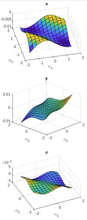
\[\oint_C (L dx + M dy) = \iint_D \bigg( \frac{\partial M}{\partial x} - \frac{\partial L}{\partial y} \bigg) dx dy\]

An example plot of the constraint curvature function for our robotic system is shown in Figure 3. If the gait cycle (drawn as a loop over this surface) moves in a positive direction (i.e. counterclockwise using the right hand rule) around regions of the surface where the curl is positive, then that means we will achieve a net positive rotation of the entire system. Similarly, if we draw a loop that moves in a negative (clockwise) direction around regions of the surface where the curl is negative, we will also achieve a net positive rotation. Overall, this plot helps us to understand what kinds of gaits will result in net displacement in x, y and \(\theta\) [1].

Figure 3 - inspired by [1]

Conclusion

I hope this post was a useful introduction to one approach for motion planning. I would recommend reading both [1] and [5] if you are curious to learn more about this topic - [5] in particular is a good in-depth explanation with several examples available for review.

References

[1] Hatton, R. L., & Choset, H. (2013). Geometric swimming at low and high Reynolds numbers. IEEE Transactions on Robotics, 29(3), 615–624. https://doi.org/10.1109/TRO.2013.2251211

[2] “Curl (mathematics).” Wikipedia. https://en.wikipedia.org/wiki/Curl_(mathematics) Visited 30 Nov 2021.

[3] “Stokes’ theorem.” Wikipedia. https://en.wikipedia.org/wiki/Stokes%27_theorem Visited 30 Nov 2021.

[4] “Green’s theorem.” Wikipedia. https://en.wikipedia.org/wiki/Green%27s_theorem Visited 30 Nov 2021.

[5] Hatton, R. L., & Choset, H. (2011). Geometric motion planning: The local connection, Stokes’ theorem, and the importance of coordinate choice. The International Journal of Robotics Research, 30(8), 988–1014. https://doi.org/10.1177/0278364910394392