In my last post, I introduced some reinforcement learning concepts that we will need to understand the policy gradient method used by MolGAN: deep deterministic policy gradient (DDPG). In this post, we are going to touch on a couple more concepts - namely actor-critic methods and off-policy approaches. Then in the next post I promise that we are going to dive into DDPG itself. I know this is taking a long time to set up but I had a lot to learn about reinforcement learning before DDPG would make sense. Let’s get started.

The Actor-Critic Concept in RL Policy Gradient Methods

Previously we saw that there are two main approaches to solving the RL problem: (1) learning and optimizing the value function and (2) learning and optimizing the policy. The actor-critic concept attempts to learn the value function and the policy simultaneously [1]. This is helpful because, as we saw with REINFORCE, we need to know the value function in order to optimize the policy. Better knowledge of the value function also helps us to reduce variance in our computation of the gradient, which is important given that we are computing the gradient as an expectation over many sampled trajectories [1].

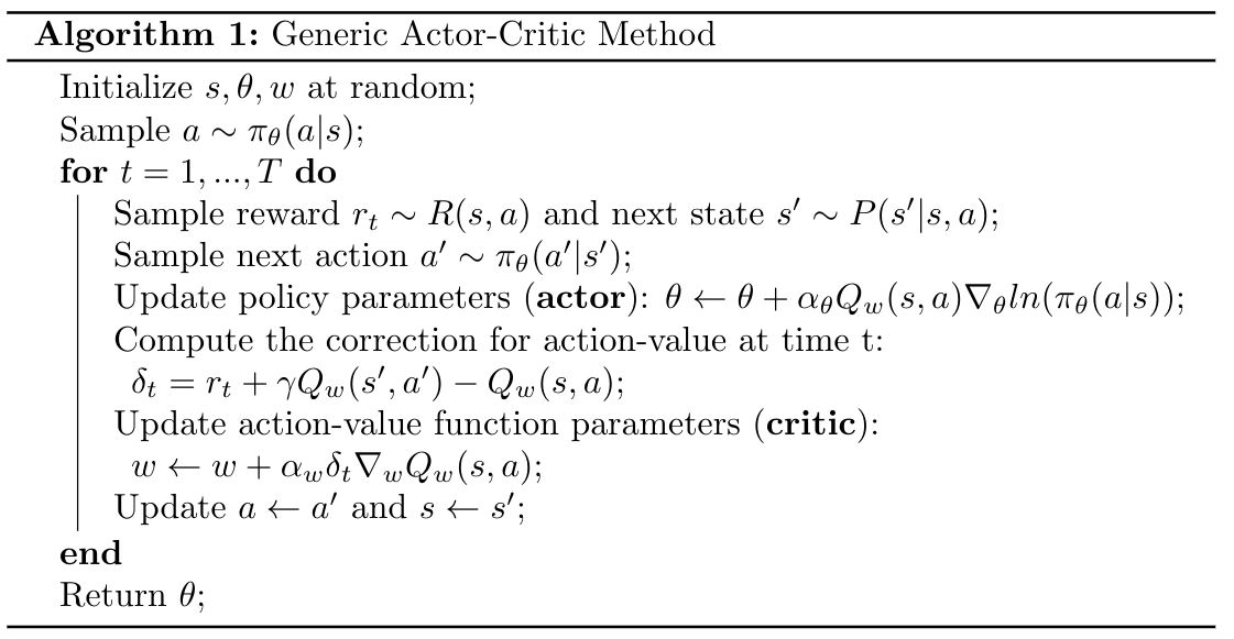
The actor-critic structure has two models: (1) the critic updates the value function parameters, w, and (2) the actor updates the policy parameters, theta, as guided by the critic [1]. Note that the critic can define the value function as either the action-value, Q, or the state-value, V [1].

Here is a very basic algorithm to show how the actor and critic work together to learn the value function and the policy simultaneously [1]:

Algorithm 1

Now that we have some intuition for how the actor-critic concept works, let’s look at how off-policy policy gradient methods work.

Off-Policy Policy Gradient Methods

In the previous post we learned about REINFORCE, which is an on-policy policy gradient method [1]. That is, we were using the target policy in the algorithm to collect samples that we used to update the parameter, theta [1]. However, in DDPG, we are going to use an off-policy approach, which has some advantages. The first is that we will not need to perform computations over the full trajectory as we did in REINFORCE [1]. Secondly, we can reuse past episodes to improve our sample efficiency (this is called “experience replay”) [1]. And thirdly, the samples we collect will not necessarily follow the target policy, which is good because it allows us to better explore the space beyond the target policy we have chosen [1].

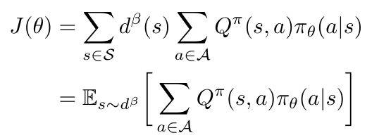
Let’s dig into the math of how we compute an off-policy policy gradient. We are going to introduce a “behavior policy” which we use to generate trajectories from which we can pull samples to estimate the gradient [1, 4]. This behavior policy is not learned, it will instead be predefined [1]. We can write an objective function to compute the reward over the state distribution that is given by this behavior policy [1]:

Equation 1

We are using beta to represent our behavior policy [1]. Notice that the Q represents the action-value function for the target policy, not the behavior policy [1]. The d term in this expression is, again, a stationary distribution, this time for the behavior policy (see our discussion about stationary distributions in the previous post) [1]. We can define d as follows [1]:

Equation 2

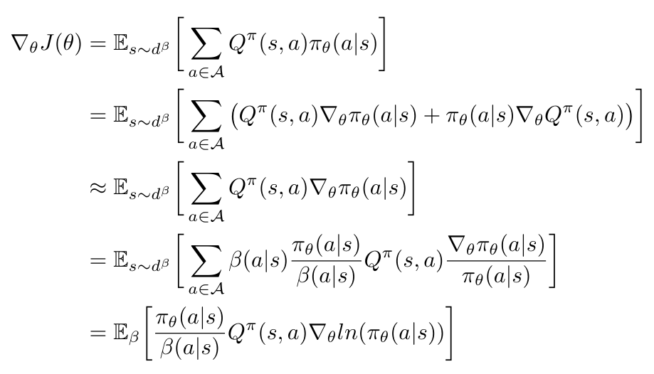
Now that we have our objective function in Equation 1, let’s write an expression for the gradient of the objective function. I’m going to show the intermediate steps as Weng does in [1], and then after we see the final expression I will add some additional commentary. Here it is [1]:

Equation 3

We begin with the same objective function we saw in Equation 1, and we first take the derivative using the product rule to get the second line [1]. Notice that the second term in the derivative, the gradient of Q with respect to theta, is very difficult to compute, and we actually choose to ignore it for the rest of the derivation [1]. There is a mathematical justification for this decision, which shows that if we approximate the gradient without that term, we are still guaranteed to reach the local minimum eventually [1]. In the fourth line we use the fact that ln(x)’ = 1/x to rewrite the right hand side, and then in the final line we recast this equation as an expectation with respect to the behavioral policy [1]. Notice that the first term in the last line is called the “importance weight,” and it gives us some degree of control over the off-policy approach [1]. The importance weight represents the balance between the target policy and the behavior policy [1].

Okay, where are we now? We have learned the actor-critic paradigm in RL, and we have seen how to compute an off-policy policy gradient method using a behavior policy to sample actions. We are almost ready to look at DDPG, but before we do, I want to introduce the idea of a deterministic policy as compared to the stochastic policies that we have seen so far. To do this, we will look at the deterministic policy gradient method (DPG) and figure out what a deterministic policy is and how it works [1].

DPG

As you’ve probably guessed, DPG is one of the precursors to DDPG, which is why we want to look at it here. The key innovation in DPG is that it uses a policy model that is deterministic, not stochastic [1]. Up to this point, we have seen policy functions, pi, that are stochastic because they represent actions as a probability distribution [1]. By changing to a deterministic model, we need to come up with a new way to calculate the gradient of the action probabilities because now we are outputting single actions instead of distributions [1]. Our new deterministic policy is [1]:

Equation 4

So how do we compute the gradient of a deterministic policy function? Let’s begin by introducing some new notation. First, we will use rho to describe the distribution over states, both initially and then at every subsequent state, after moving k steps per some policy which we call mu (this is called the “visitation probability density”) [1]. We can also use rho to describe the discounted state distribution [1]. All of these expressions are given as follows [1]:

Equation 5

Okay, so now that we have rho and mu, we can write a new objective function for our deterministic policy [1]:

Equation 6

Compare this expression to Equation 1 - do you see the similarities? In essence, we have simply replaced pi with rho. Now that we have a new objective function, let’s compute its gradient. The deterministic policy gradient theorem tells us that if we apply the chain rule, we get the following equation [1]:

Equation 7

We can plug the result of Equation 7 into any of our existing policy gradient frameworks that we’ve seen before. Weng notes that using a deterministic policy in an on-policy policy gradient method can reduce the amount of exploration we see, because we have removed the stochasticity from our approach [1]. There are two solutions to this - we can either add noise to the deterministic policy (thereby making the policy stochastic again) or we can use an off-policy method where the behavior function gives us the stochasticity we need to explore [1].

Since DDPG is an off-policy approach, let’s preview how we could use the deterministic policy gradient theorem in a generic off-policy approach. To do so, let’s say that we have a stochastic policy, beta, and our state distribution is described with respect to this policy [1]. We have the following objective function and corresponding gradient [1]:

Equation 8

Okay, I think we finally have all the pieces we need to understand DDPG. In my next and (hopefully) final post on this topic, we will look at how DDPG actually works.

References:

[1] Weng, L. “Policy Gradient Algorithms.” Lil-Log. 8 Apr 2018. https://lilianweng.github.io/lil-log/2018/04/08/policy-gradient-algorithms.html Visited 04 Aug 2020.

[2] N. De Cao and T. Kipf, “MolGAN: An implicit generative model for small molecular graphs,” arXiv Prepr. arXiv 1805.11973, May 2018.

[3] Lillicrap, T., Hunt, J., Pritzel, A., Heess, N., Erez, T., Tassa, Y., Silver, D., and Wierstra, D. “Continuous Control with Deep Reinforcement Learning.” arXiv Prepr. arXiv 1509.02971, Sept 2015.

[4] Emami, P. “Deep Deterministic Policy Gradients in TensorFlow.” 21 Aug, 2016. https://pemami4911.github.io/blog/2016/08/21/ddpg-rl.html Visited 05 Aug 2020.