I was recently introduced to the concept of factor graphs and I am interested in using them in my research. I’m going to take a two-step approach to learning about factor graphs this time: first, we are going to look at what a factor graph is and some of its key advantages, as explained by the excellent blog posts by Prof. Frank Dallaert’s group at Georgia Tech. Then I am going to dive in deeper by reviewing a paper written by Dallaert and Kaess [4] that gives a more thorough discussion of using factor graphs to perform simultaneous localization and mapping (SLAM). My hope is that this first post will give us enough of the big picture and some of the mechanics that reading the paper will make more sense than it would otherwise. Okay, let’s give this a go!

What are Factor Graphs?

Simply stated, factor graphs are bipartite graphical models containing nodes that are either variables (unknown quantities) or factors (functions operating on subsets of the variables) [1]. Factor graphs are of interest to many fields for three primary reasons [1]:

• They are flexible, and can be used to model many different problems.
• They lay out the underlying structure of the problem which helps to find ways of solving the problem efficiently (we will see this with an LQR example).
• They help researchers think about the problem by laying it out as a combination of variables and factors.

Dallaert explains that factor graphs are very useful in solving optimization problems. One example of where factor graphs shine is in solving the simultaneous localization and mapping (SLAM) problem in robotics [1]. In SLAM, we are trying to learn (1) a map of our environment and (2) our position within this map [2]. (We’ve seen this topic before when discussing filters.) To solve SLAM, we can use information from a wide variety of sensors, including LiDAR, IMU’s, and camera data. We then compute the probability that we are at a certain location on the map given the measurements taken from these instruments. More specifically, we compute the maximum a posteriori (MAP) estimate (which combines both a prior and a likelihood estimate) of our current location [1]. A factor graph can be used to lay out and solve this problem because it can represent the measurement data as variables, and the function for computing the MAP as a factor.

Another benefit to factor graphs is that not all variables are connected to all factors. An example of a factor graph is shown in Figure 1. As you can see, some variables feed into certain factors, while other variables do not. This is useful because it captures the idea that many factors are local - in other words, that a particular function may only depend on a few relevant variables from among all the data that we have [1]. For example, in SLAM, our location at a given time is calculated using the data collected in the most recent time step, but it doesn’t directly draw from all the data in all previous time steps. The estimate of our position is dependent locally on the most recent measurement data [1].

Now that we have given a brief explanation for what factor graphs are and where they can be useful, let’s use one to solve the LQR problem*1.

Solving LQR with Factor Graphs

Before I start, let me just say that the explanation provided by Dallaert’s group is much more thorough than mine and I would highly recommend reading their post in detail.

The goal of using this example is to show 1) how we can lay out a problem as a factor graph and 2) how we can leverage the factor graph structure to efficiently compute the solution to the LQR problem [3]. Just as a reminder, the linear quadratic regulator (LQR) is a state feedback controller that is applying an optimal gain to a system, where optimality is defined by a cost function that considers the costs of state and control errors in the control policy [3]. Mathematically, this can be written as [3]:

Equation 1

We are going to use this to find the optimal gain, K, such that it produces the optimal control policy [3]:

Equation 2

Let’s consider a situation where we are trying to optimize u over three time steps. We can draw the graph as shown in Figure 1 [3]. Notice that the cost function and the dynamics are factors, drawn in blue, and the state and control inputs are variables, drawn in green. As we step through time, we can see that there are factors that compute the cost of the state and the control inputs at every time step, and a factor that computes the state at the next time step.

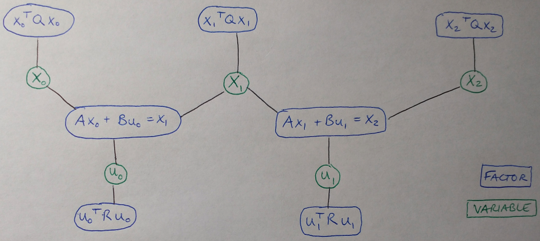
Figure 1

Now that we have this layout, we can sequentially eliminate variables until we find a set of recurrence relations to solve for K [3]. Variable elimination is a key algorithm that allows us to speed up the computation of the factor graph [4], so we are going to look at it in detail in the next section.

Variable Elimination with Factor Graphs

Again, Dallaert’s group’s post on variable elimination with factor graphs is a much cleaner explanation, so please feel free to check out their post. But if you’re sticking with me, let’s start by looking at how we can eliminate a state, x2 (one of the variables shown in green in Figure 1). We look at the two factors connected to the state x2 and our goal is to rewrite them in terms of other, earlier states and controls. These factors are shown in red in Figure 2. We can observe that it is possible to write x2 in terms of x1 and u1, and we can substitute that into both factors in red [3]:

Equation 3

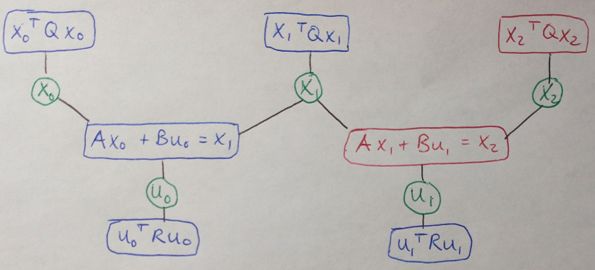
Figure 2

Now we can eliminate x2 because we don’t need it to perform the computations represented by the factors in red. I replace x2 in Figure 3 with the dynamics equation giving x2 in terms of x1 and u1. Note that I’ve written the replacement for x2 in black, and there are two directed edges coming into this new node. This signifies that the dynamics constraint replacing x2 is a node in a Bayes network*2 [3]. I’ve also added a new node for the cost factor of x2, as shown by the red and blue box in Figure 3.

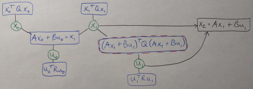
Figure 3

Now the next thing that I want to do is eliminate a control, u1, from the graph. I am going to do this by replacing the two factors connected to u1, shown in red in Figure 4, with a new cost factor on x1 and an equation for the optimal control, u1*(x1).

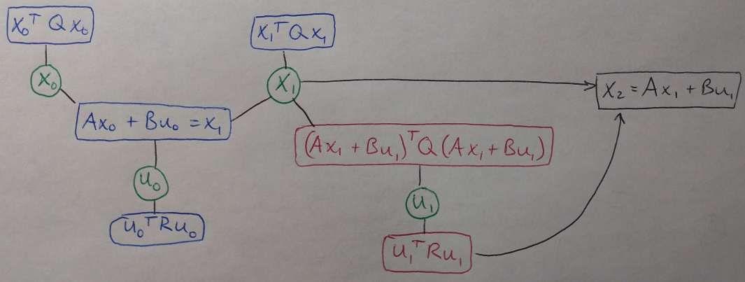
Figure 4

I can write the combined cost of the two red factors as follows [3]:

Equation 4

This expression, phi3, is the optimal action-value function (remember our discussion about reinforcement learning for this concept). We want to minimize this cost in LQR control, so we can take the derivative of phi3 with respect to u1, and set the derivative equal to zero. In other words [3]:

Equation 5

Now I can substitute this expression for the optimal control, u1*(x1) back into our expression for phi3 to get a new cost factor that operates on x1 only, and does not explicitly involve u1 (which we are trying to eliminate). This looks like so [3]:

Equation 6

And now I can replace u1 with a new node in the Bayes network, and I have created a new factor shown in Figure 5 in red and blue.

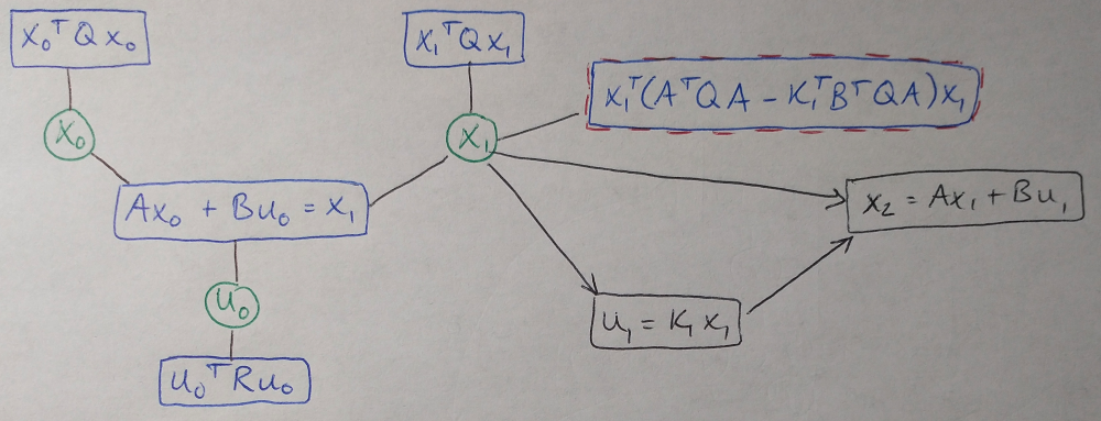
Figure 5

This process of eliminating states and controls continues until the entire factor graph has been converted into a Bayes network [3]. We observe that, in general, we can write the following expression (or recurrence relation) for K [3]:

Equation 7

The expressions given in Equation 7 are exactly the discrete algebraic Ricatti equations! I think this is a really cool result - using just a graphical format for the problem of LQR, and some algebra, we were able to derive the Ricatti equations! The final Bayes network is shown in Figure 6. In essence, it is a graphical representation of the control law: u = Kx [3].

Figure 6

Okay, so we have made a lot of progress so far - we have been introduced to factor graphs, learned how to lay them out, used them to derive the solution to the LQR problem and learned how to perform variable elimination over a factor graph. Whew!

There is one more thing that I wanted to cover before moving on to Kaess and Dallaert’s paper, and that is how variable elimination relates to factorizing matrices and solving the least squares problem. But I think that might be too much information for one post, so instead I will put up a new post shortly that focuses on matrix factorization and solving the least squares problem. Until then, thanks for reading.

Footnotes:

*1 I still need to write a post on how to solve the LQR problem using Ricatti equations, I will try to get that out soon.

*2 A Bayes network (or belief network) is a probabilistic graphical model that is a directed, acyclic graph [5]. It is used to show conditional dependencies between nodes like the one shown below.

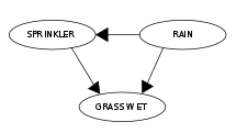
Figure 7 - Source: [5]

References:

[1] Dallaert, F. “What are Factor Graphs?” GTSAM Posts. 01 Jun 2020. https://gtsam.org/2020/06/01/factor-graphs.html Visited 15 Feb 2021.

[2] “Simultaneous localization and mapping.” Wikipedia. https://en.wikipedia.org/wiki/Simultaneous_localization_and_mapping Visited 15 Feb 2021.

[3] Chen, G., Zhang, Y., Dallaert, F. “LQR Control Using Factor Graphs.” GTSAM Posts. 07 Nov 2019. https://gtsam.org/2019/11/07/lqr-control.html Visited 15 Feb 2021.

[4] Dellaert, F., & Kaess, M. (2006). Square root SAM: Simultaneous localization and mapping via square root information smoothing. International Journal of Robotics Research, 25(12), 1181–1203. https://doi.org/10.1177/0278364906072768

[5] “Bayesian network.” Wikipedia. https://en.wikipedia.org/wiki/Bayesian_network Visited 15 Feb 2021.