Today I was working through a dynamic programming problem in Leetcode when I encountered a reference to an algorithm that I had not heard of before: Kadane’s Algorithm. I wanted to write a quick post to explain this algorithm in more detail, and hopefully this will help me solve more Leetcode problems, too. I’ll start by describing the problem that Kadane’s Algorithm solves, and some of the contexts where it appears in practice. Then I will describe a number of ways to solve it, including Kadane’s Algorithm.

The Problem

Kadane’s Algorithm solves what is known as the maximum subarray problem, where we are given an array of numbers, and we want to find the continuous subarray with the largest sum. The numbers in the array can be positive, or negative, or 0. As an example, if we are given the array [1]:

[−2, 1, −3, 4, −1, 2, 1, −5, 4]

Then the solution is [4, -1, 2, 1] = 6.

This might seem like an arbitrary, esoteric problem (which is how I feel about most of Leetcode’s questions, if I’m being honest) but this problem actually turns out to have many real world applications. The problem was originally formulated by Ulf Grenander as a way of computing the maximum likelihood estimate for patterns in images. He wanted to find a 2D array with the maximum sum within an image, and formulated this 1D version as a way of looking for the underlying structure in the problem. Grenander found an algorithm that ran in $\mathcal{O}(n^2)$ time (which is $n$ times slower than the fastest possible approach, which would only need to scan the array once and would therefore, theoretically, run in $\mathcal{O}(n)$ time). Another researcher, Michael Shamos, found a $\mathcal{O}(n \log (n))$ solution, and talked about this problem and his search for faster algorithms during a seminar he presented at Carnegie Mellon University. Jay Kanade, a professor in the Department of Statistics, heard the seminar and apparently developed a solution in $\mathcal{O}(n)$ time in under a minute [1, 2].

Apocryphal stories aside, solving the maximum subarray problem is useful to more than just finding patterns in images. For example, this kind of problem appears in genomic sequencing work where we are often trying to find specific regions in protein sequences that have certain properties, or we are looking for GC-rich regions in DNA strands. And it turns out that there is more than one way to solve the maximum subarray problem. We can solve it using divide-and-conquer strategies (like Shamos), using dynamic programming, or brute force [1].

Kadane’s Algorithm

Before presenting Kadane’s Algorithm, it might help to consider some properties of this problem to become more familiar with it.*1 Specifically [1]:

1. If the input array has all positive numbers, then the solution is easy - it’s just the sum of all the numbers in the array.

2. If the input array has all negative numbers, then we want to find the maximal single entry in the array and just return that value.

3. It is possible for there to be more than 1 subarrays with the same maximum value.

Kadane’s Algorithm is an elegant approach to solving this problem, which works given all of these properties of the problem statement. We will consider here the formulation of the problem where empty subarrays are not allowed. In this case, we can write Kadane’s Algorithm as follows [1]:

def max_subarray(numbers):
    best_sum = float('-inf')
    current_sum = 0
    for x in numbers:
        current_sum = max(x, current_sum + x)
        best_sum = max(best_sum, current_sum)
    return best_sum

Kadane’s Algorithm is employing a simple form of dynamic programming, because it is building up a solution from optimal solutions to sub-problems. The sub-problem is finding the maximum sum for the subarray that we have seen at the previous step. That is, the current_sum is the optimal solution to the sub-problem of finding the max sum of the subarray that represents all the numbers we have seen up to now [1].

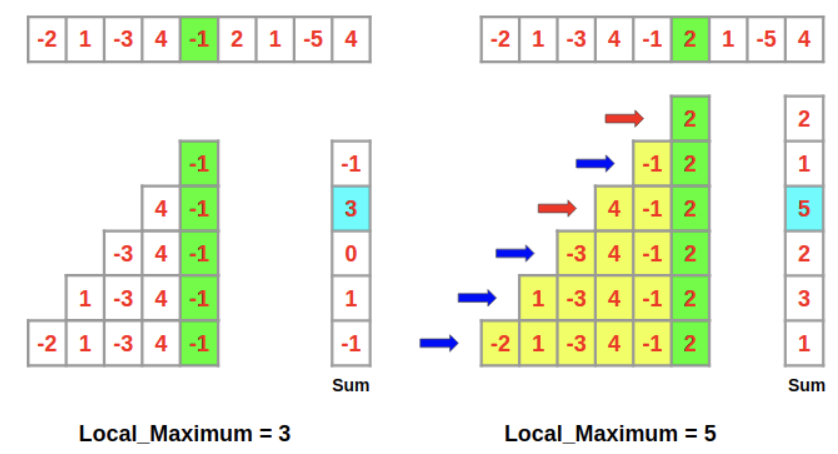
Rohit Singhal gave a very nice diagrammatic explanation of the dynamic programming aspect of this algorithm, as shown in Figure 1 [3]. If we consider the left hand side of Figure 1, we can see that we can find the optimal solution to the maximum subarray at nums[4] by finding the local maximum among all the possible subarrays. Once we know that the local maximum is 3, we carry that information forwards to solving the next sub-problem: the maximum subarray at nums[5]. At nums[5], we don’t need to completely redo all the summation calculations for the sums of the subarrays - we can just add the value of nums[5] = 2 to the local maximum of the previous step, that is we can add 2 + 3 = 5.

Figure 1 - Source [3]

Footnotes

*1 One thing I am trying to get better at while solving Leetcode problems is taking the time to really think about the problem, and to play around with solving a couple numerical examples by hand, before coding up a solution. I think it’s probably better in the long run to think my way to the right answer instead of coding/debugging my way to a poorly-implemented answer.

References

[1] “Maximum subarray problem.” Wikipedia. https://en.wikipedia.org/wiki/Maximum_subarray_problem Visited 4 Sept 2022.

[2] “Joseph Born Kadane.” Wikipedia. https://en.wikipedia.org/wiki/Joseph_Born_Kadane Visited 4 Sept 2022.

[3] Singhal, R. “Kadane’s Algorithm — (Dynamic Programming) — How and Why does it Work?” Medium. 31 Dec 2018. https://medium.com/@rsinghal757/kadanes-algorithm-dynamic-programming-how-and-why-does-it-work-3fd8849ed73d Visited 4 Sept 2022.