In this blog post I want to describe the basics of linear time invariant (LTI) systems.

Figure 1

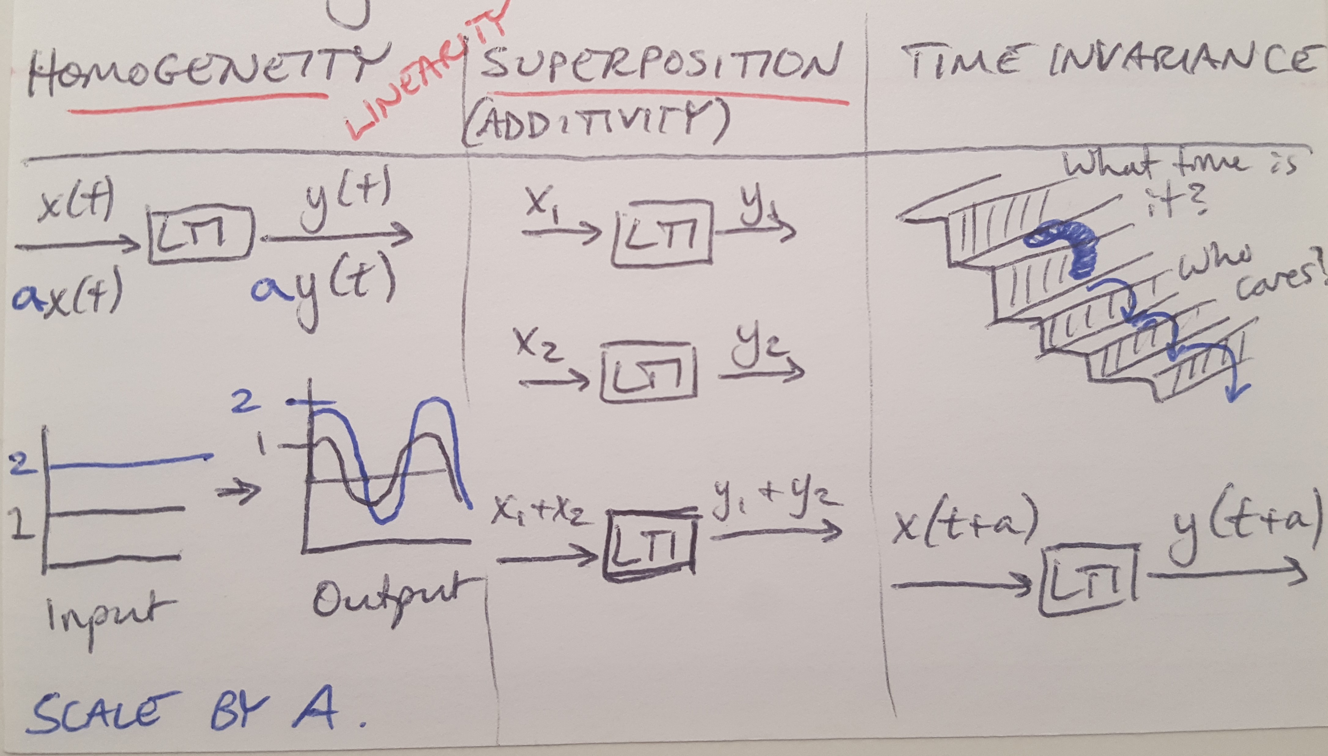
All LTI systems have three properties, as listed below and depicted in Figure 1 [1]: (1) Homogeneity
(2) Superposition
(3) Time Invariance

Homogeneity states that you can scale a system by a constant factor (so if you double the input, the output also doubles) [1]. Superposition states that if you add two inputs together, the output is the sum of the outputs of the individual inputs [1]. Together the homogeneity and superposition criteria define the requirements for a linear system [1].

Time invariance states that a system will behave the same way no matter what point in time an action occurs [1]. Inputs translated in time will produce the same output translated in time [1]. This property makes a linear system also time invariant.

No real world system is truly time invariant, but the concept makes it easier to solve problems. The hardware used in a control system usually has some amount of nonlinearity in its dynamics, which is why this is an abstraction [1]. Often we can work within a small range where the hardware has a more linear behavior [1].

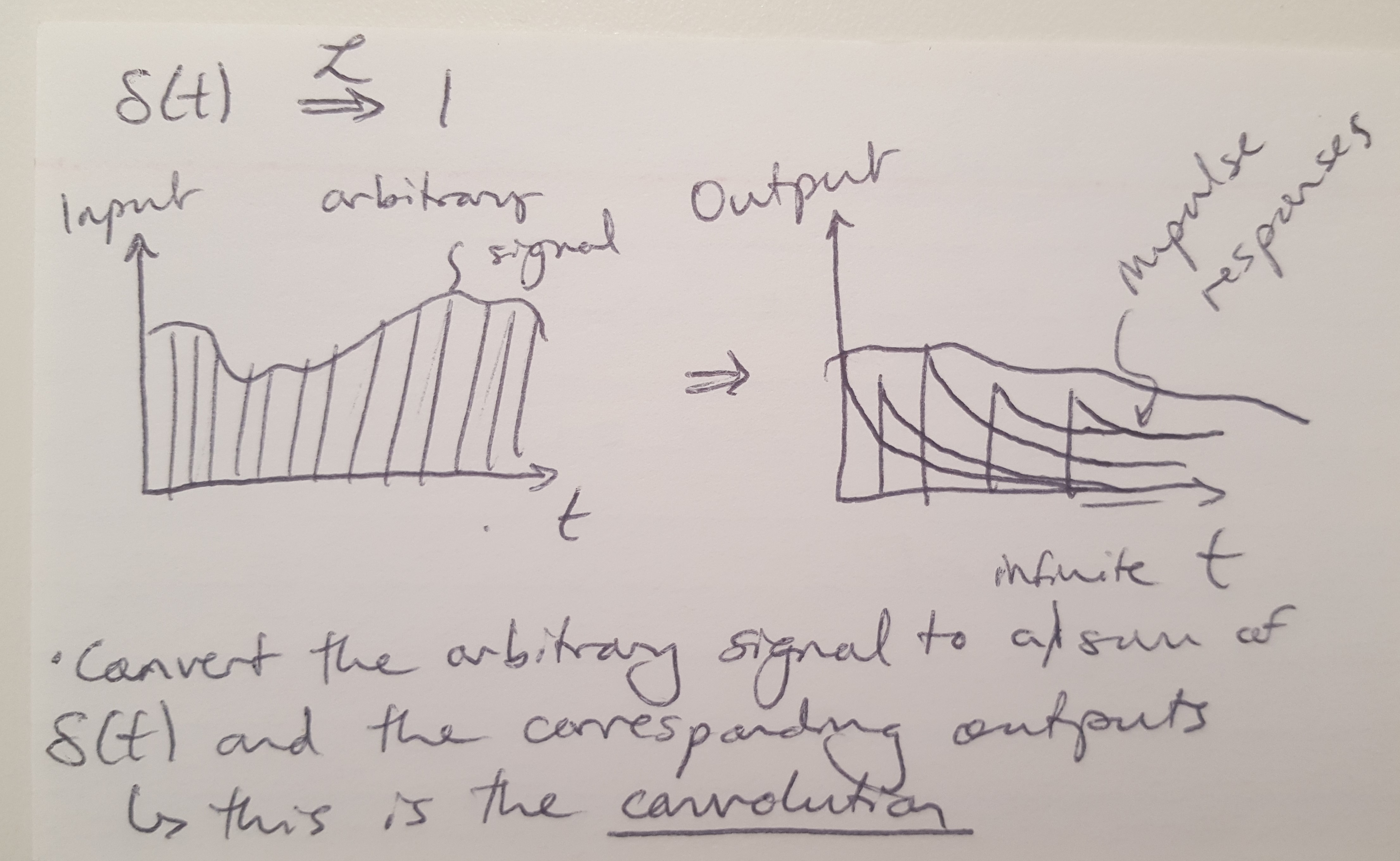
Why is it so important to work with linear systems in classical control theory? There are many reasons, but one of them is that we write transfer functions to describe systems in classical control, and these transfer functions only work if we assume that the systems are linear [1]. One way to define a transfer function is to say it is the Laplace transform of the impulse response of an LTI system with no initial conditions [1]. To write a system’s response to an impulse, or any input, we can write it as a sum of a series of impulse responses, see Figure 2 below [1]. This is easiest if we transform the input and the response to the frequency domain with the Laplace transform [1]. Then we can write the system’s response as a multiple of impulse responses [1].

Figure 2

What we have just described above is called “convolution” in the time domain, and it is equivalent to multiplication in the frequency domain [1]. Mathematically, we can define convolution as a mathematical operation that combines two functions to produce another function that shows how the two inputs changed each others’ shapes [2]. In this case, we are using convolution to understand how the system’s response can be made to look like a series of impulse responses. And thanks to the Laplace transform, convolution in the time domain is equivalent to multiplication in the frequency domain.

I am still working to understand this thoroughly, but for now I will close with the equation for convolution in the hopes that this helps clarify things [2].

References

[1] Douglas, Brian. “Control Systems Lectures - LTI Systems.” https://www.youtube.com/watch?v=3eDDTFcSC_Y&list=PLUMWjy5jgHK1NC52DXXrriwihVrYZKqjk&index=4 Visited on 08/14/2019.

[2] Wikipedia. “Convolution.” https://en.wikipedia.org/wiki/Convolution Visited on 09/09/2019.