In practicing for quals last week I managed to get myself very confused about linearization, so I wanted to go back to fundamentals. In this post I will cover why we linearize, the basic concept behind it, and the equations for Jacobian linearization, which is a standard method for linearizing. As it turns out, I’m still a little confused about the particular example that started me down this road in the first place, so hopefully in the near future I will return with another post that straightens that issue out. But for now, let’s begin with the stuff I do understand.

In the real world, there is no such thing as a linear time invariant (LTI) system [1]. All systems have some nonlinearities in them and often we can see this manifested in their dynamics equations [1]. But we like to work with linear systems for 3 main reasons, namely [1]:

(1) Linear systems are easier to understand. We can quickly grasp their dynamics and stability characteristics.
(2) We have tools for linear system controller design already, and we like to use them.
(3) It can be faster to simulate a linear system than a nonlinear system, which is advantageous when we are testing hardware, especially fast embedded controllers.

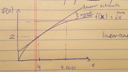
So given our preference for LTIs, we must find a way to approximate a nonlinear system into a linear system in some limited way, as demonstrated in the equation above. That is the process of linearization. As an example, consider the plot of f(x) below, where the function is the square root of x [1]. This is a nonlinear function but we can pick some point and draw a straight line approximation about that point. The point we choose is called the operating point, or the equilibrium point [1]. And the line is our linear estimate. As long as our system will be operating close to the operating point (for example if our operating point is 4, and our system will be running in the range of x = [3.9, 4.1]), we can assume that our linear estimate will return values sufficiently close to the true values that we can effectively control our system [1]. If we try to operate far from our operating point (say x = [2, 6]) then we probably cannot assume that our linearization will be effective for that entire range [1].

Figure 1

We use Jacobian linearization to obtain a linear approximation for our nonlinear system as follows [1]:

Notice that xbar and ubar are our operating points. This expression looks like the equation for a line, y = mx + b, because we have our y-intercept, the value of xdot at xbar and ubar, and we have our slopes as determined by the changing state and the changing input [1].

This is all I am going to say about linearization for now (I realize it’s not a lot) and hopefully come back soon with more information.

References

[1] Douglas, Brian. “Trimming and Linearization, Part 1: What is Linearization?” MATLAB. https://www.youtube.com/watch?v=5gEattuH3tI Visited 09/16/2019.