Logistic regression is a form of classification, which is a kind of supervised learning [1]. Logistic regression differs from linear regression because it fits a sigmoid function to the data set, instead of fitting a straight line [1]. (The sigmoid function is going to appear again when we discuss neural networks because it is used there as well [2].) In this post we will discuss when logistic regression is useful, the mathematics of the algorithm and how to implement it on a simple dataset.

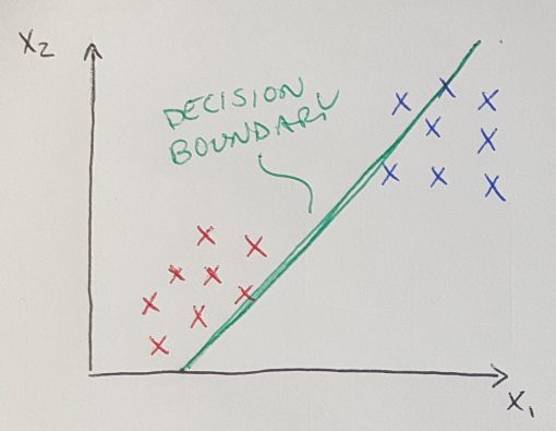
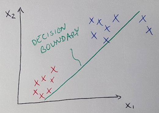
As previously mentioned, logistic regression (like linear regression) is a form of classification - specifically binary classification, where we are trying to differentiate data into two distinct classes [1]. Logistic regression is often used when linear regression fails to adequately distinguish data into two distinct classes [1]. Consider the example below [1]. In Figure 1, linear regression is able to define a line (called the decision boundary) that demarcates the separation between the two binary classes we are using to classify the data set. But now consider Figure 2, where a new data point is added to the dataset, and it is an outlier located far to the right. In this case, a linear regression algorithm will be pulled in the direction of this outlier, and it will (incorrectly) classify the blue data points as red data points. Logistic regression is designed to resolve these kinds of situations [1].

Figure 1

Figure 2

The logistic function, as defined by Verhulst* in the 1800s [3], is also described as the sigmoid function [2] and can be defined by the following equation [2]:

Equation 1

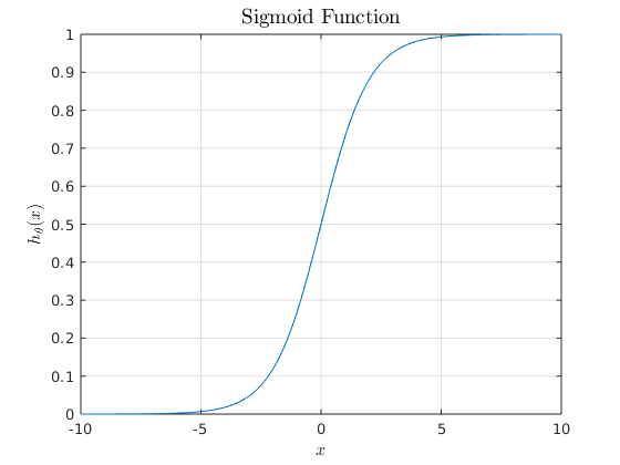
Where theta represents the vector of fit parameters, and x is the input data [2]. The shape of this function is shown in Figure 3. We use “h” to represent the function because we are going to use this function as our hypothesis in logistic regression [1]. That is, our hypothesis now states that if the argument of the hypothesis is greater than 0, then the hypothesis returns y = 1 (i.e. it categorizes the data as “true”) and if the argument of the hypothesis is less than 0, the hypothesis returns y = 0 (i.e. it categorizes the data as “false”) [1]. Notice that this kind of function will not fall prey to outliers like linear regression does - additional data points on the extremities of the dataset will not change the shape of the function.

Figure 3

The argument to the hypothesis is also called the decision boundary [1]. It is written as [1]:

Equation 2

Notice that this is only an example inequality that could represent the decision boundary. We could choose any polynomial, with higher order terms, if we thought it would better separate the two classes [1]. We will use gradient descent to choose the parameters, theta, to fit the decision boundary to the dataset so that the hypothesis accurately models the training data [1].

Just as with linear regression, in logistic regression we need to fit the parameters, theta, to the dataset, and we will do this with gradient descent [1]. If you recall from my previous post, gradient descent takes the derivative of a cost function and follows the slope of the cost function to find the global minimum. In other words, gradient descent looks for the values of theta that minimize the cost function, so that the hypothesis function returns an output that is as close as possible to the training data.

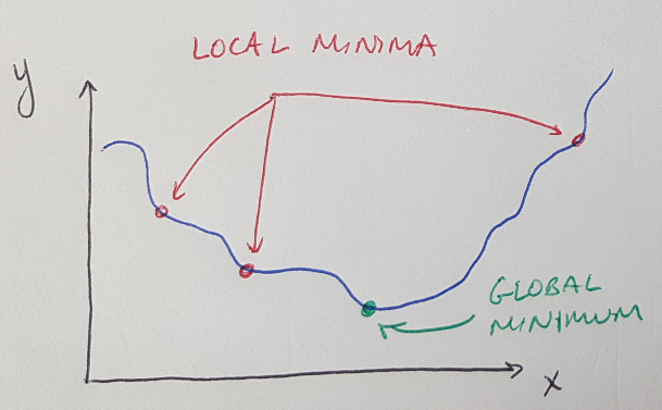
Figure 4

If we were to use the same cost function for logistic regression as we used for linear regression, we would find that, because of the nonlinear nature of the sigmoid function, the cost function would become non-convex [1]. Non-convex functions have multiple local minima, and therefore it can be difficult to find the global minimum because our gradient descent algorithm may get stuck in a local minimum instead (see Figure 4) [1]. So to avoid this problem, logistic regression uses a logarithmic cost function which, when used with the sigmoid function as the hypothesis, will return a convex cost function [1]. This ensures that we will find the global minimum using gradient descent [1]. The logarithmic cost function is [1]:

Equation 3

We can actually simplify this function to one equation as follows [1]:

Equation 4

And when we take the derivative of the cost function, we will find that we actually get exactly the same expression as we found when we performed linear regression [1]. The important distinction, of course, is that the hypothesis has changed from a linear function to the sigmoid function [1]. We can write the equation for gradient descent as [1]:

Equation 5

Where the hypothesis, h, is the sigmoid function in this case. Notice that there are more advanced optimization algorithms than the standard gradient descent approach we have seen thus far [1]. A lot of these methods use a line search algorithm, which means that they search for the best value of alpha (the learning rate) to use on each iteration, which can make them more efficient than standard gradient descent, which uses a fixed learning rate [1].

This approach can also be used for categorizing data into multiple classes (i.e. “multiclass classification”) [1]. To use logistic regression to sort data into multiple groups, we learn decision boundaries that separate each group from all of the rest of the data (this is called the “one vs. all” approach) [1]. We then place new data in the group that returns the highest value from its hypothesis function [1].

*According to [3], Verhulst never explained why he chose the term “logistic” for this function. There is some speculation that it might have been chosen in contrast to a logarithmic curve [3].

References:

[1] Ng, A. Machine Learning course, week 3 lecture notes on logistic regression. https://www.coursera.org/learn/machine-learning/supplement/QEYX8/lecture-slides Visited 04/06/2020.

[2] Wikipedia. “Sigmoid function.” https://en.wikipedia.org/wiki/Sigmoid_function Visited 04/06/2020.

[3] Wikipedia. “Logistic function.” https://en.wikipedia.org/wiki/Logistic_function Visited 04/06/2020.