In DNA nanotechnology, there is a rapidly growing collection of software tools for simulating how nanoscale DNA structures will appear when fully formed and at equilibrium. I have been learning to use tools for conducting these molecular dynamics simulations in my research. I wanted to write about the theory behind these simulations. My goal is to become more knowledgeable about how to intelligently leverage simulation in my research, and also to be aware of its limitations.

This post will focus on the theoretical underpinnings of molecular dynamics (MD) simulations, and will be heavily informed by an excellent paper by Bopp et al. titled “The Hitchhiker’s guide to molecular dynamics” [1]. Let’s start by introducing MD simulations and why they’re useful.

What are Molecular Dynamics Simulations?

The term molecular dynamics refers to a computer simulation approach for modeling the motion of particles (such as atoms or molecules). The computer simulates the motion of a large number of particles (the system) over a period of time, showing how the system evolves [2]. The details of how the computer conducts these simulations for many particles are the focus of this blog post. Note that for the purposes of this discussion, we are assuming that all of the simulations we want to run are for unconstrained systems at equilibrium [1].

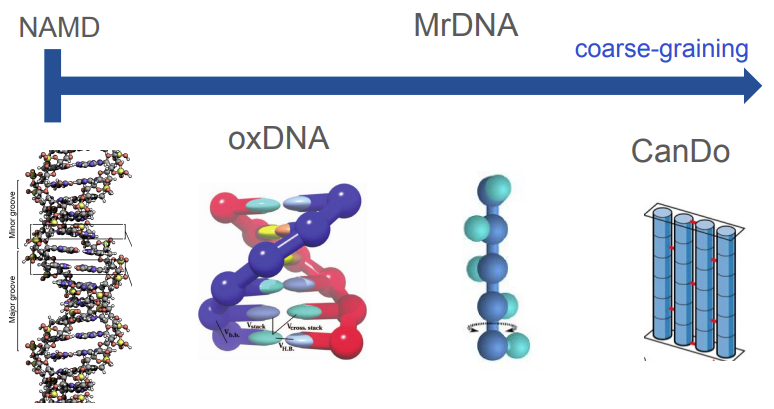
The DNA nanotechnology research community uses MD simulations to predict what a nanoscale DNA structure will look like at equilibrium. There are a wide range of tools available for simulating structural configurations of DNA constructs, and not all of them are considered MD simulations. Consider Figure 1 below, where we can see that there are a range of modeling tools available from very coarse-grained tools to fine-grained MD simulations. Some of the more coarse-grained tools, like mrDNA, abstract away some of the details of the DNA helix, instead representing structures as a series of rigid mechanical elements [3]. Using these low-resolution representations of DNA allows mrDNA to run very rapidly and return an analysis to the user quickly. Conversely, high resolution tools like NAMD are all-atom simulations, which means that they consider each atom in the DNA helix individually during runtime [3].

Figure 1 - Source [10]

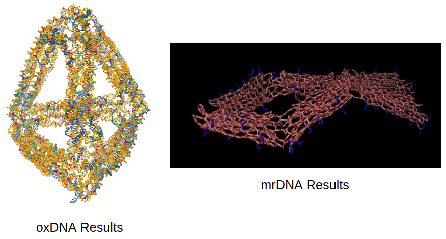
I have used several of these tools so far, including mrDNA (on the coarse-grained end of the spectrum) and oxDNA (falls in the middle of the spectrum, more detailed than mrDNA but coarser than NAMD) [10]. I have added some example outputs from each tool below to help give you an idea of what these simulations look like. In addition to giving the user a visual representation of the structure’s shape, it is also possible to pull other information from the simulation, like how far a particular element moved over time, or the root-mean-square of the fluctuations of all the individual elements from their mean position. We will discuss the analysis in more detail later. But first, let’s talk about the fundamental theory that is common across all the simulation tools we have discussed here.

Figure 2

The Basics of Classical Statistical Mechanics for MD Simulations

Molecular dynamics (MD) simulations are based on classical statistical mechanics1 (because this approach is based on classic or Newtonian mechanics2). The basic idea behind classical statistical mechanics is that we can characterize a system macroscopically using just a few state variables, even though there are a huge number of microscope states that the particles in the system could be in at any given time. Imagine a glass of water as a system of water molecules: I can tell you the temperature and pressure of the water in the glass to describe the state of the entire system. But you could also characterize the system by describing the position and velocity of each water molecule in the glass. We would also call the positions and velocities of each molecule as the state of that system [1].

It would take an inordinate amount of time to represent all of the states of the water molecules in the glass. So when we conduct MD simulations, we only simulate a sample of molecules, while trying to ensure that we have chosen enough molecules to get a good representation of all the possible states of the system [1]. An MD simulation solves Newton’s equations of motion over many time steps for this sample of particles, given some set of external conditions (such as temperature or pressure) [1].

The Potential Energy Surface

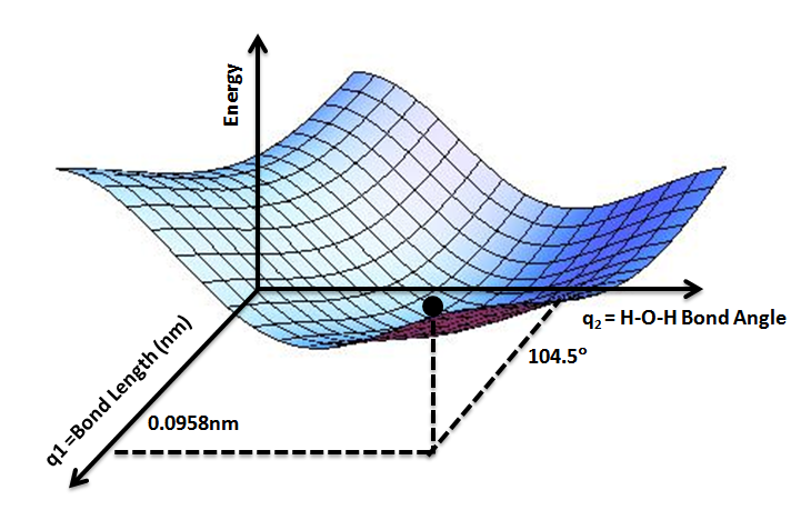
MD simulations use an energy-based approach to computing the states of particles, and in general we make the assumption that we can derive the energy of a given particle from a Potential Energy Surface (PES) [1]. See Figure 3 for a conceptual illustration of a PES. Briefly, a PES is a function that describes the energy of a system in terms of certain parameters, often the positions of the elements of the system [4]. We call it a “surface” because if you consider a function with two parameters, then the values of the energy output by the function can be visualized as a surface, as shown in Figure 3 [4].

Figure 3 - Source [11]

So now we can characterize this model of our system by choosing a set of parameters we will use to quantify the PES. We have two choices of model: first, we can use the NVE model, which has N particles in a system, contained inside a fixed volume V, and having some constant total energy, E [1]. It is also possible to use a second model called the NVT model, which also has N particles in a volume V, but replaces the energy with temperature, T [1]. (You can also have an NpT model which replaces the constant volume with a constant pressure [1].)

We generally prefer to use the NVE model for MD simulations [1]. To understand why, let’s recall that MD simulations use the initial conditions of the system’s particles (i.e. their initial position and velocity) and Newton’s equations of motion (or Lagrange or Hamilton approaches) to compute the particles’ trajectories over time [1]. As the simulation performs these calculations, it assumes that energy is conserved. Energy conservation means that the total energy in the system does not change, and the NVE model is also making that assumption. So in this way we can see that using the NVE model fits well with our classical mechanics approach to simulating the individual particles in our system [1].

We can compute properties for the system at a given time step, and compute an average over all time to obtain bulk properties [1]. We call these properties observables (or measurable quantities), and in general we can compute them as [1]:

Equation 1

Where {q, p} is the sample as represented by all the particle trajectories, q, and the momenta of all the particles, p, at some time t-i, where i ranges from 1 to some final step, M [1]. The function A describes some property of interest that we calculate for some moment in time. The value represents the thermodynamic average of A over time for a fixed set of conditions (i.e. temperature, pressure, density, etc.) [1].

Interaction Models

In reality, it is really difficult to compute the PES for a system, especially in real time during a simulation run [1]. To make things easier, we typically use an interaction model to approximate the PES [1]. There are many different kinds of interaction models in use today, but Bopp et al. categorize them into two sets: fundamental models and ansatz models [1]. A fundamental model is intended to be an accurate representation of the physics driving the interactions between particles [1]. They are often built using robust approximations for quantum chemical energies [1]. The second set of models, ansatz models*3, are designed to fit the model to some desired result [1].

According to Bopp et al., simulation tools often combine fundamental and ansatz approaches to build a composite interaction model [1]. They warn that using both approaches allows the interaction model greater flexibility, but also makes it easier for the model to stray from the physical reality it is trying to represent [1]. As a result, Bopp et al. recommend looking at trends in the results of a simulation, instead of the absolute values, because it is very difficult to fit the model well enough to the physical system to generate truly accurate results [1].

There are many types of models for particle interactions, and Bopp et al. suggest that many of these models can be used in either the fundamental or ansatz approach as described above [1]. We will discuss some of these models here, because some of them are used in the DNA nanotechnology tools that I commonly use [1]:

• Pair potentials are functions that describe the potential energy between two objects that interact [8]. They are actually a class of model because there are many different functions that can be used to represent this potential energy, including Coulomb’s law, Newton’s law of gravitation and the Lennard-Jones potential*4 [8].

• All-atom vs united atoms are two approaches to modeling molecular structures [1], as we discussed above in the introduction. An all-atom model represents each atom individually, whereas a united atom model will abstract groups of atoms into single entities [1]. These single entities can be rigid, semi-flexible or flexible depending on what is appropriate for the situation [1].

• Bond-order potentials capture the directionality of chemical bonds (also called reactive potentials) [1]. Bond-order potentials can account for changes in the topology of molecules which allows molecules in the model to dissociate [1].

The Importance of Equilibrium and Equilibration

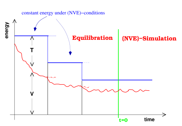
Now that we have a fundamental understanding of how an MD simulation works, we need to highlight the importance of equilibration [1]. What do I mean by that? When you set up a simulation and start running it, it is likely that the initial configuration of your structure will have too much potential energy [1]. That is, some of the nucleotides may be too close to each other, inducing repulsive potential energy, and others may be too far away, inducing an attractive potential energy. Therefore, you need to give the simulation time to shift the particles enough to allow the system to actually reach equilibrium (remember that equilibrium is often one of the lower-energy states of the system) [1]. This idea is also illustrated in Figure 4.

Figure 4 - Source [1]

The MD simulation will often have a built-in relaxation process that allows the system to reduce its potential energy [1]. The relaxation process may need to iteratively relax the structure because as the potential energy is decreased, the kinetic energy of the system particles may increase [1]. The simulation will need to scale down the resultant velocities accordingly to avoid simply oscillating between high potential and kinetic energies [1]. Overall this relaxation process is also called the equilibration process and we should not include it in our final results or analysis [1]. Instead, once we can see that the system has actually arrived at equilibrium*5, we should now run the simulation for some time and analyze those results obtained at equilibrium, and not before [1].

When and Why You Should Use MD Simulations

One thing I love about the paper by Bopp et al. is that it clearly lays out the two situations where you should use MD simulations in your research. I don’t know if I am the only person who struggles with this, but I frequently reach for MD simulations before I have thought through why I need them. Usually my reasoning is something vague like “I want to see what it has to tell me” or, if we’re being really honest, “I bet a simulation of this structure would look cool.” I struggle to come up with concrete questions or analyses that I want to conduct using an MD simulation, and so I end up wasting a lot of time because as a result, I run a simulation without thinking about whether it’s appropriate for the situation or if the results will actually help me.

Bopp et al. tell us that there are two reasons why you should run an MD simulation: for analysis and for prediction [1]. The first reason, analysis, refers to situations where you have obtained some result, or made some observation, in an experiment, and you want to develop an explanation for that result [1]. For example, you might be trying to build a two-dimensional tile structure with DNA origami, and your atomic force microscopy (AFM) images show that the structure is curved. You run a simulation to compare your staple routing to one used in a reference paper, and you might find that indeed your staple routing is different and thus causes the tile to curve more than the staple routing used by the authors of the reference paper.

In the second case, we use MD simulations to predict what will happen before we go to the bench to do an experiment [1]. This can be especially useful if each experiment is time-consuming or expensive, and we want to limit the number of experiments we conduct. We can use MD simulations to predict the configuration of a specific structure design and try to optimize the design on the computer before we build it at the bench.

You should also keep in mind the limitations inherent in MD simulations. There is a trade-off in MD simulations between the simulation time you can accommodate and the number of particles you want to model [1]. That is, you will increase the wall time*6 of your simulation if you try to study a phenomenon over a long time scale (more than a few milliseconds), or if you try to study a very large number of particles [1]. This is important because if you want to use the MD simulation to analyze why your DNA origami structure fell apart after an hour, this will be very difficult because MD simulations usually are not designed to run for such long time scales. Another example where you will hit these limitations is if you are trying to model an enormous DNA structure, because you may find that it takes longer to simulate than it would to build experimentally.

Some Practical Advice

Before we close out this post, Bopp et al. offer some practical advice and potential pitfalls to avoid when running MD simulations, including [1]:

• Unit confusion - pay attention to the units used in your particular software tool and make sure that any values you enter into the model are in the correct units.

• Time step - choosing a simulation time step is a trade-off between computational cost and accuracy. Specifically, if the time step is large, that will reduce the total number of time steps required and it will be cheap to run the simulation. However, larger time steps may cause the trajectory calculations to miss events in the integration scheme, causing the simulation to diverge from what we would expect to see. The general rule of thumb offered by Bopp et al. is to choose a time step between 1/25th and 1/10th of the total simulation time, T. They recommend running an equilibrium simulation at your chosen time step and checking to see if the system remains at equilibrium or if integration error accumulates and causes the system to diverge from equilibrium over time.

• Backup often - save your files frequently and maintain a backup on a secondary platform.

Conclusion

With that I think we have covered most of the main points of Bopp et al.’s introduction to molecular dynamics simulations. I think there is a lot more to learn so I will continue to post as I encounter new concepts. In the immediate future, I will be adding a post specifically describing the way oxDNA works, including its interaction model, fitting parameters and some best practices.

Footnotes:

*1 Where does the “statistical” come from? It refers to the fact that we are computing the trajectories for a large number of particles, and then using statistical analysis to analyze the distribution of states over all the particles. When you learn about mechanics in high school physics, you are usually thinking about a single element with a single state (i.e. a ball has one state at one time step because it is a single element) [5]. But in statistical mechanics, we introduce the statistical ensemble which you can think of as many virtual copies of the system, where each copy has a different state [5]. The statistical ensemble, in other words, represents the probability distribution over all the possible states of the system [5].

*2 If you are reading this and saying “but what about using quantum mechanics, wouldn’t that be better for modeling atoms?” then Bopp et al. have a note for you. You are right, quantum mechanics would also work but classical mechanics (as represented by the PES) are an acceptable approximation for quantum mechanics assuming that we are operating at or above 300K [1].

*3 The term ansatz refers to a strategy in mathematics of assuming the form of some unknown function, and then fitting that form to reproduce known outcome [7]. When we fit a line to a set of data, our ansatz is the equation for a line, and it represents our assumption that the data represents some linear relationship [7].

*4 The Lennard-Jones potential (aka the LJ potential aka 12-6 potential) is a pair potential between two molecules, often used in modeling water [9]. It accounts for soft repulsive and attractive interactions between electronically neutral particles [9]. The equation for the Lennard-Jones potential is [9]:

Equation 2

Where r is the distance between the particles, epsilon is the depth of the potential well adn sigma is the distance at which the energy, V, is zero [9].

*5 I feel obligated to point out, like Bopp et al. did, that it can be difficult to identify equilibrium. There are necessary, but not sufficient, conditions for equilibrium - that is, even if a system satisfies all the properties of equilibrium, it does not prove that the system is actually at equilibrium [1]. It could, instead, be at a metastable state that will take a very long time to exit (if it exits at all) [1].

*6 “Wall time” is geek speak for the elapsed real time that it takes for a computer program to run [6].

References:

[1] Bopp, P. A., Hawlicka, E., & Fritzsche, S. (2018). The Hitchhiker’s guide to molecular dynamics: A lecture companion, mostly for master’s and PhD students interested in using molecular dynamics simulations. ChemTexts, 4(1), 1–16. https://doi.org/10.1007/s40828-018-0056-1

[2] “Molecular dynamics.” Wikipedia. https://en.wikipedia.org/wiki/Molecular_dynamics Visited 05 Jan 2021.

[3] K Doye, J. P., Fowler, H., Prešern, D., Bohlin, J., Rovigatti, L., Romano, F., Šulc, P., Kui Wong, C., Louis, A. A., Schreck, J. S., Engel, M. C., Matthies, M., Benson, E., Poppleton, E., & K Snodin, B. E. (n.d.). The oxDNA coarse-grained model as a tool to simulate DNA origami.

[4] “Potential energy surface.” Wikipedia. https://en.wikipedia.org/wiki/Potential_energy_surface Visited 06 Jan 2021.

[5] “Statistical mechanics.” Wikipedia. https://en.wikipedia.org/wiki/Statistical_mechanics Visited 06 Jan 2021.

[6] “Elapsed real time.” Wikipedia. https://en.wikipedia.org/wiki/Elapsed_real_time Visited 06 Jan 2021.

[7] “Ansatz.” Wikipedia. https://en.wikipedia.org/wiki/Ansatz Visited 06 Jan 2021.

[8] “Pair potential.” Wikipedia. https://en.wikipedia.org/wiki/Pair_potential Visited 06 Jan 2021.

[9] “Lennard-Jones potential.” Wikipedia. https://en.wikipedia.org/wiki/Lennard-Jones_potential Visited 06 Jan 2021.

[10] Taylor, R. “Dynamic Nanomachines: Workshop on coarse-grained simulation tools mrDNA and oxDNA.” Lecture notes from 24-684: Special Topics: Nanoscale Manufacturing Using Structural DNA Nanotechnology, Fall 2020.

[11] By AimNature - Own work, CC BY-SA 3.0, https://commons.wikimedia.org/w/index.php?curid=29213158 Visited 06 Jan 2021.