Gain and phase margins are a useful concept to understand when designing controllers using Bode plots. Today I am going to explain what they are and how we can find them on both a Bode plot and a Nyquist plot. If we have time, I will go into how the margins are related to the sensitivity function.

Recall that when we pass a sinusoidal signal through an LTI system, the system can change the signal’s amplitude (gain) and angle (phase). The Bode plot displays these changes at every frequency. The phase and gain margins of a system define the amount of extra gain and phase we have in our design that prevents us from moving into instability. The less margin we have, the less stable our system is. Why is this important? Controls engineers try to have gain and phase margins built into their designs because the real world implementation of their controllers never perfectly matches up with the system model, and these safety margins allow us to guarantee stability at all frequencies regardless of the real world process variations. Just to give you some examples, process variations can come from many sources, like:

(1) Unexpected rotor inertia - affects system gain
(2) Temperature sensitive power sources - affects system gain
(3) Bearing drag - affects gain and phase
(4) Computer delays - affects phase

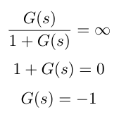
Let’s look at how we determine the gain and phase margins. Recall that we typically analyze the open loop transfer function because it is easier to analytically find its poles and zeros. What characteristics of the open loop indicate that the closed loop system will trend toward instability? One indication is if the gain of the closed loop system goes to infinity, then the closed loop system will be unstable. Mathematically, that is expressed as G(s) = -1 (gain = 0dB) as shown below. If the phase is -180 degrees, this will also drive the system to instability because it will cause a sign change, just as G(s) = -1 causes a sign change. Putting these two conditions together, if there is any point on the Bode plot where the gain is 0dB and the phase is -180 degrees, then we know the closed loop system is unstable at that frequency!

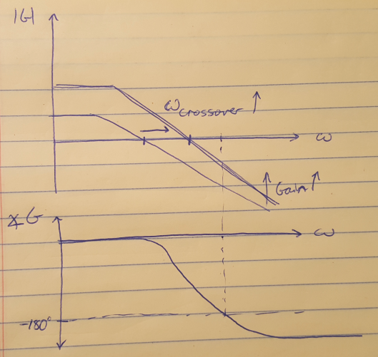
Therefore, we can say that the gain and phase margins tell us how far we are from gain = 0dB or phase = -180 degrees. Let’s examine the gain margin in detail first. Recall that as we increase system gain, it shifts the magnitude Bode plot upwards. It also moves the crossover frequency to the right. Typically, as the crossover frequency moves to the right, the crossover frequency approaches the frequency where the phase is -180 degrees, see Figure 1 below). The gain margin tells us how much we can increase the gain before the crossover frequency overlaps the frequency where the phase is -180 degrees.

Figure 1

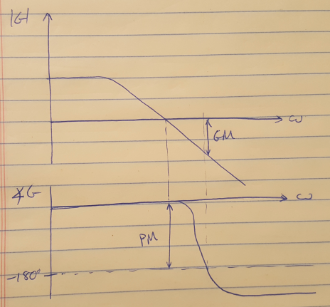
Similarly, the phase margin is defined as the amount of phase at the crossover frequency available above -180 degrees (see Figure 2 below). Note that if the phase never crosses -180 degrees, then the gain margin is infinite. Also be aware of how your entire Bode plot looks - you may have peaks and troughs in your curves that take you very close to the 0dB line or the -180 degree line, which can lead to instability in the system.

Figure 2

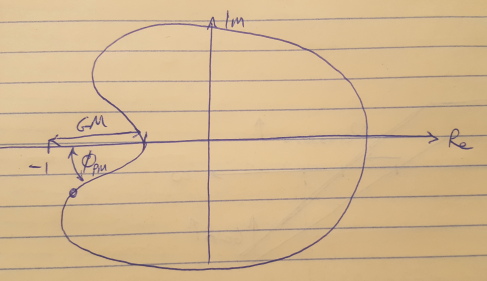
We can also plot the gain and phase margins on a Nyquist plot as shown in Figure 3. In this case, the gain margin is the distance from the curve to the -1 point on the real axis. The phase margin is the angle between the point on the curve closest to -1, to the point -1.

Figure 3

It is possible that your Nyquist plot will come veeeeeery close to -1. If this is the case, we would like to identify the situation mathematically. We can say that we want to calculate the distance between the open loop transfer function and -1 for all frequencies, and then find the minimum distance. We invert this metric as shown below so that we are trying to maximize the inverse of the distance to -1 to try to find the most sensitive point on the Nyquist plot. This math is shown below.

References

[1] Douglas, Brian. “Gain and Phase Margins Explained!” https://www.youtube.com/watch?v=ThoA4amCAX4&list=PLUMWjy5jgHK1NC52DXXrriwihVrYZKqjk&index=31 Visited 09/16/2019.

[2] Douglas, Brian. “Understanding the Sensitivity Function.” https://www.youtube.com/watch?v=BAWdZvF1O40&list=PLUMWjy5jgHK1NC52DXXrriwihVrYZKqjk&index=32 Visited 09/16/2019.