Machine learning has interested me for a couple years, ever since I read Pedro Domingos’ book, The Master Algorithm. In the lab, we have been discussing reinforcement learning lately and I have been trying to teach myself about this topic. This post is going to be my first introduction to reinforcement learning, and I hope to follow it with more posts soon.

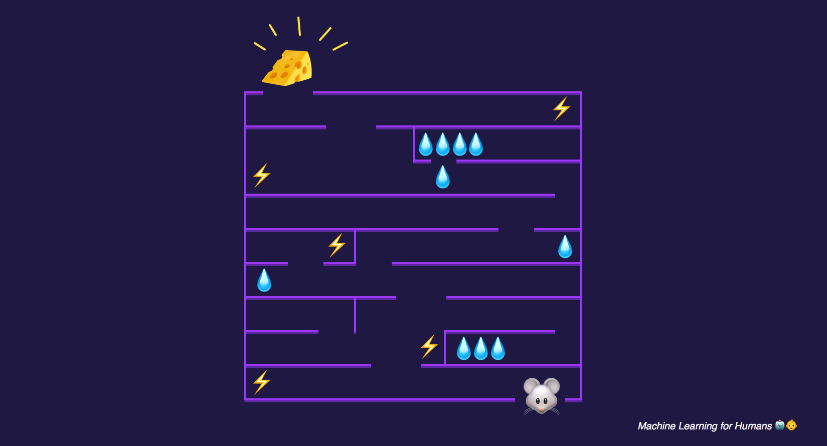
Reinforcement learning is a subcategory of machine learning. It uses a combination of rewards and penalties to make the computer solve a problem on its own [1]. Many of the references listed here use a maze with rewards in it and a goal at the end as an example of the kind of problem that reinforcement learning is good at solving (see Figure 1) [3]. The designer writes a reward function that encourages the computer to find rewards, and to look for the goal, but does not tell the computer how to find rewards or the goal. The computer learns to search the maze on its own, without guidance from the human designer. The computer is trained over hundreds of thousands of iterations to solve the same kind of problem, and on every iteration it improves its solution. Ultimately, the great power of reinforcement learning is that the computer can run through this maze thousands more times than a human could in their entire lifetime [2-3]. Reinforcement learning research has exploded recently because we can leverage new powerful hardware tools like GPUs and parallel processing to iterate much more rapidly than was ever previously possible. This is one of the reasons why reinforcement learning can be used to play Go and beat the greatest human Go players: the computer can play more rounds of Go than a human can in their whole life, and so will eventually learn more strategies than a human will ever know [1-2].

Markov Decision Processes

I’m going to introduce terminology slowly because machine learning is overflowing with new vocabulary. In this section, I’m going to introduce the fundamental concept of Markov Decision Processes (MDPs) because it is a good foundation of how to think about reinforcement learning in general. In a Markov Decision Process, there is an actor; in reinforcement learning, the actor is the computer [3]. The actor is present inside some environment; in our maze example, the maze is the environment [3]. The actor is in a specific state at any given point in time [3]. At the start of trying to solve the maze puzzle, the actor is located at the entrance to the maze, and so its current state is at the start location. The actor can take different actions, such as going left, right or forward in the maze [3]. Every time the actor performs an action, it transitions to a new state [3]. The environment also returns a reward for that specific action - for example, if the actor comes across a piece of cheese after turning right in the maze, it will receive a reward for finding the cheese [2-3].

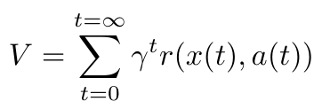
In addition to getting an immediate reward, the agent is also calculating a value function [3]. This value function calculates the expected long term reward that the agent predicts it will get from a certain set of actions. The value function is shown below [3]:

Equation 1

The gamma term is called the discount factor, and it represents the difference between current and future rewards [3]. For example, if the actor is going to receive a reward of 4 in two moves, and the discount factor is 0.5, then the value of that reward to the actor right now is 1 (see math below). Notice that the reward function is dependent on the current state and action. Also notice that the reward is not dependent on prior states or actions. This idea is called “memorylessness”, and it simply means that your current reward and your future expected rewards do not depend on your past choices, except in the sense that they have gotten you to your current state [3]. Everything you need to know about the past is encoded in information about where you are now. It is not necessary to keep track of all your past decisions while solving a problem.

Equation 2

Q-Learning and Policy Gradients

Reinforcement learning is based on an MDP model, but it needs something more than just a reward or value function to help the agent decide what actions to take. The agent needs to be able to learn an optimal control policy because the human designer will not directly tell the agent what to do. In reinforcement learning, there are two categories of approaches to determining the optimal control policy for a given agent and environment. The first is called Q-learning, and the second is called policy gradient.

Q-learning maps a certain state-action pair to an expected value for that pair [3]. That is, it returns the expected value for choosing a certain action in the current state as well as choosing the optimal action in the next state. Let’s consider the equation for the Q function [3]:

Equation 3

The function starts with the previous Q-value for a particular state-action pair (presumably calculated during the last learning iteration, or, if this is the first learning iteration, it is fixed at some arbitrary constant) [3]. We update the previous Q-value with a second value that is modulated by the learning rate, alpha. The learning rate is used in many places in machine learning, and it determines how aggressively we update the previous Q-value with the new information we have just learned. If alpha is 0, it means that we don’t update the previous Q-value at all [3]. Conversely, if alpha is 1, it means that we will essentially replace the previous Q-value with a new value, and we won’t consider any of the information contained in the old value at all [3]. The reward, r, is the reward for the current action-state pair and is given to us by the reward function that the human algorithm designer has supplied. The discount factor, gamma, performs the same function as described above in the section on MDPs, and this time it is modifying the estimate of the optimal future value, which is the next term in the expression. The estimate of optimal future value calculates the maximum achievable reward for all available actions at the next time step [3]. Finally, we subtract the previous estimate of the Q-value for this state-action pair to make sure the function is only updating the Q-value based on the difference between the old and new estimates [3].

Okay, that was a lot to handle, but the key takeaway is that the Q-function is a way of choosing the best current action based on how big the expected reward is for the actions in the next state. Policy gradients are also designed to help the agent choose the best current action, but the policy gradient approach is slightly different from the Q-function. The Q-function is trying to predict the best action to take based on what reward it will return in the next state. In contrast, the policy gradient learns a policy function which maps the state to the best action for that state [3]. Do you see the difference? The policy gradient is a slightly more straightforward method which simply asks: this is the state I am in now, what is the best choice I can make if I only care about the reward I get right now? Instead, the Q-function considers the next state as well as the current state when picking the best action to take.

Exploration vs Exploitation

So far, we have talked about using policy gradient and Q-learning approaches to choose the best actions for the agent, with an emphasis on maximizing rewards. But is that always the best thing to do? In reinforcement learning, there is a balance between encouraging the agent to explore or exploit an environment [3]. Exploiting an environment refers to what we have already been discussing - looking “greedily” for the maximum reward in every state. We want to exploit the environment to maximize our rewards. You might be wondering why this is a bad thing - isn’t the entire purpose of reinforcement learning to maximize the reward function that the human algorithm designer has written? Consider a maze like the one shown below. It might be that there are rewards for finding the water and energy, and they are not in the same direction as the cheese at the end of the maze. If the agent is too focused on maximizing reward, it may continue looking through the maze for more water and energy, instead of looking for the cheese. But if we encourage the agent to also explore, then the agent will sometimes choose actions that do not maximize rewards, but do allow it to venture into new parts of the environment that it hasn’t seen before. This is good when the goal is not close to the rewards in the maze.

Figure 1 (source: [3])

Deep Neural Networks

The policy gradient and Q-function approaches to solving the reinforcement learning problem are both implementations of very complicated functions. Many researchers use neural networks as function approximators for these approaches [2-3]. The neural networks themselves tend to have many (>3) layers to account for the complexity of the functions they are approximating, so we call them deep neural networks [2-3]. When we used deep neural networks to solve reinforcement learning problems, we call the approach deep reinforcement learning. My next post will explore neural networks in more depth because they are a very cool tool in their own right.

References:

[1] B. Osinski and K. Budek. “What is reinforcement learning? The complete guide.” deepsense.ai. https://deepsense.ai/what-is-reinforcement-learning-the-complete-guide/ Visited 12/02/2019.

[2] C. Nicholson. “A Beginner’s Guide to Deep Reinforcement Learning.” skymind.ai. https://skymind.ai/wiki/deep-reinforcement-learning Visited 12/05/2019.

[3] V. Maini. “Machine Learning for Humans, Part 5: Reinforcement Learning.” https://medium.com/machine-learning-for-humans/reinforcement-learning-6eacf258b265 Visited 12/04/2019.