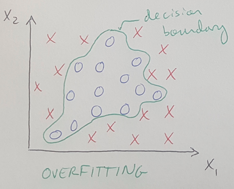
I just want to write a brief post about overfitting and how we can try to deal with it using regularization. Overfitting occurs when our model can accurately predict the outcome for the training data, but it does not accurately predict outcomes for new data it has not seen before [1]. This happens because the algorithm has used a higher-order polynomial to draw a decision boundary, which very precisely matches the dataset but also produces a very irregularly shaped decision boundary which may not accurately model the true difference between the two datasets, see Figure 1 below [1].

Figure 1 - Inspired by [1]

To avoid overfitting, we can use regularization to make our hypothesis better match the data [1]. Regularization reduces the weight that some of the fitting parameters, theta, have in the hypothesis, which tends to simplify the hypothesis and therefore generate a better model [1]. We can do this by adding a term to our cost function that reduces all of our fitting parameters according to some factor, called the regularization parameter, or lambda [1]. This extra regularization term has the effect of smoothing out our hypothesis function, which reduces the amount of overfitting in the model [1].

Equation 1

Notice that, by convention, we do not regularize the parameter theta_0 [1]. Once we modify our cost function, we also have to modify our gradient descent algorithm. If we update the gradient descent equation (for all fitting parameters AFTER theta_0), then we see that we get this new expression [1]:

Equation 2

This expression can be re-written as [1]:

Equation 3

Notice that the coefficient of theta_j in the first term is very close to 1, if alpha is small [1]. This coefficient will have the effect of slightly shrinking theta_j before we also decrement theta_j by the same amount that we would using standard gradient descent that we’ve seen before. So ultimately, regularization does not affect gradient descent very much at all. Notice that as lambda increases, the amount that we decrement theta_j also increases. But if we increase lambda by too much, it will too heavily weight all of the theta terms in the cost function (except for theta_0) [1]. This will force the gradient descent algorithm (which is trying to minimize the cost function) to significantly minimize the values of theta to compensate for their increased weight [1]. This will look like the algorithm is underfitting the model, because it will essentially only have a theta_0 term left, which will draw a horizontal line regardless of the dataset [1].

This approach works the same way for both linear and logistic regression, although of course the hypothesis is different in each case [1]. The additional term for regularization in the cost function is also different for linear logistic regressions.

References:

[1] Ng, A. Machine Learning course, week 3 lecture notes on regularization. https://www.coursera.org/learn/machine-learning/home/week/3 Visited 02 May 2020.