We first encountered the reparameterization trick when learning about variational autoencoders and how they approximate posterior distributions using KL divergence and the Evidence Lower Bound (ELBO). We saw that, if we were training a neural network to act as a VAE, then eventually we would need to perform backpropagation across a node in the network that was stochastic, because the ELBO has a stochastic term. But we cannot perform backpropagation across a stochastic node, because we cannot take the derivative of a random variable. So instead, we used something called the reparameterization trick, to restructure the problem. In this post, I am going to go into this solution in more detail. First I will outline why we need the trick in the first place, and then I will try to provide more insight into the mathematics behind the reparameterization trick.

Why Do We Need the Reparameterization Trick?

As I mentioned in this introduction, I learned about the reparameterization trick in the context of developing variational autoencoders, so I will focus on that application here. However, it is worth noting that the reparameterization trick can be applied to a wide variety of distributions and functions, and it is used in multiple places besides VAEs [1].

In a variational autoencoder, we are trying to learn an approximation of a posterior distribution, p(z given x), which converts the input data, x, to a latent space representation, z. We are doing this by learning an optimal approximation of p(z given x), which we call q*. I can optimize q* by minimizing a loss function using gradient descent - in other words, by using backpropagation to teach a neural network to represent q*. But the problem we run into when we do this is that we cannot take the derivative of one particular term in our loss function. The loss function can be written as follows [2]:

Equation 1

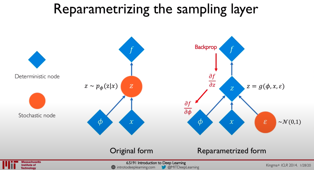
The first term in the loss function is stochastic with respect to z, because z is a random variable [3]. I cannot take the derivative of a random variable, so the backpropagation algorithm will get stuck at this node in the neural network [3]. Consider the left-hand side diagram in Figure 1, where the stochastic node (in orange) is acting as a bottleneck, preventing us from backpropagating the derivatives from f to phi and x [3]. I can use the reparameterization trick to restructure this part of the neural network so that I have a deterministic node representing z, which provides a clear path for the backpropagation algorithm to convey information from f to phi and x, as shown in the right-hand side of Figure 1 [3].

Figure 1 - Source [3]

So in short, the reparameterization trick allows us to restructure the way we take the derivative of the loss function so that we can take its derivative and optimize our approximate distribution, q* [3]. In the next section, I will give a mathematical grounding for the reparameterization trick.

The Math Behind the Curtain

In the last section we saw that the reparameterization trick somehow converts the representation of the random variable, z, into a deterministic part and a stochastic part [3]. Let me just solve the mystery right away and say that the reparameterization trick rewrites the representation of z as a random variable into the following expression [1]:

Equation 2

The first term in the reparameterized version of z - specifically, mu - is deterministic and so we can take the derivative of z. The standard deviation is still stochastic, but that’s okay, because it is no longer along the critical path in our backpropagation chain [3]. But why can we do this?

The goal of reparameterization is to find a way to recast a statistical expression in a different way while preserving its meaning [1]. The reparameterized expression has to be equivalent to the original, but by writing it in a different form, we are often making it possible to look at the expression in a new way, and we can use new tools to work with it [1].

Reparameterization is a method of generating non-uniform random numbers by transforming some base distribution, p(epsilon), to a desired distribution, p(z; theta) [1]. The transformation from the base to the desired distribution can be written as g(epsilon ; theta), as follows [1]:

Equation 3

The transformation must be some combination of simple operations, like addition, multiplication, logarithmic functions, exponentials and trigonometric functions [1]. The base distribution, p(epsilon), must also be easy to sample from [1]. We then use these basic functions to transform the base distribution to the desired distribution [1]. There are three primary approaches to building this transformation, g(epsilon ; theta) [1]:

(1) Inversion. If we know the cumulative density function (cdf) for the desired distribution, p(z ; theta), then we can simply invert it and apply it to the base distribution [1]. In this approach, the base distribution must be a uniform distribution so that it will take on exactly the cdf of the desired distribution [1]. This approach also assumes that the cdf is invertible [1]. Given the simplicity of this approach, it is quite popular [1].

(2) Polar Coordinate Transformation. This method can be used to represent a pair of values pulled from a random variable (we can also call these random variates) in polar coordinates [1]. For example, if we had pulled (x, y) from p(z; theta), we could rewrite them as (r cos(theta), r sin(theta)) [1]. The reason we would want to do this is that it enables us to use other sampling tools to work with these random variates that we could not use otherwise [1].

(3) Coordinate Transformation. More generally than polar coordinates, these methods use shifting and scaling transformations (i.e. addition and multiplication) to transform a base distribution [1]. This approach is perhaps the simplest of the three we have seen here, and it is the transformation that we use to reparameterize a normal distribution [1].

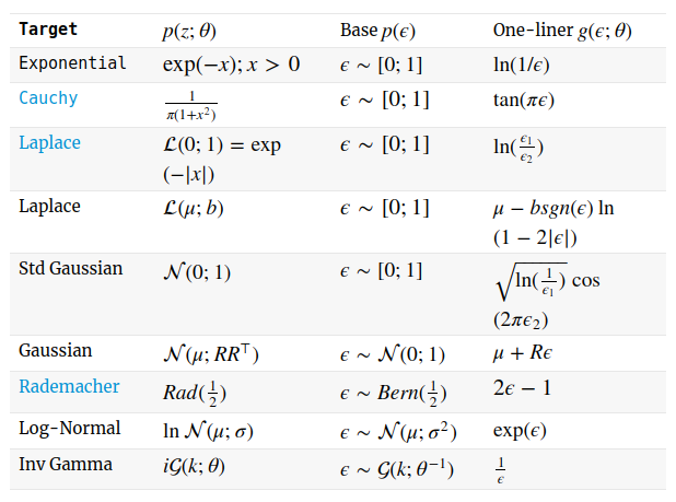
It is worth noting that there are ways to reparameterize lots of different expressions, not just the normal distribution [1]. These reparameterizations are often called “one-liners” because it takes one line to convey the reparameterization* [1]. Some other commonly used reparameterizations are shown in Figure 2. These reparameterizations are also easy to find in many software packages, so don’t bother writing your own functions [1].

Figure 2 - Source [1]

Hopefully this explanation provides a little more context for where the reparameterization trick comes from, and that you can understand why we might want to use it. I want to leave you with one final comment: the reparameterization trick works very well as long as you are using continuous distributions. However, it will not work for discrete collections of points; I will be writing soon about the Gumbel-softmax distribution, which was developed to deal with this problem, so stay tuned.

Footnotes:

*The term “one-liner” comes from a 1996 paper that developed these reparameterizations for many different distributions [1]. The paper was written by Luc Devroye and can be found here [1].

References:

[1] Mohamed, S. “Machine Learning Trick of the Day (4): Reparameterisation Tricks.” The Spectator, Shakir’s Machine Learning Blog. 29 Oct 2015. http://blog.shakirm.com/2015/10/machine-learning-trick-of-the-day-4-reparameterisation-tricks/ Visited 26 May 2020.

[2] Altosaar, J. “Tutorial - What is a variational autoencoder?” https://jaan.io/what-is-variational-autoencoder-vae-tutorial/ Visited 06 May 2020.

[3] Soleimany, A. “Deep Generative Modeling, MIT 6.S191.” MIT Introduction to Deep Learning 6.S191: Lecture 4. 28 Feb 2020. https://www.youtube.com/watch?v=rZufA635dq4 Visited 26 May 2020.