We are going to bounce around a couple different controls topics in these next posts, I’m sorry for not choosing a more logical order. Please bear with me!

Today we are going to talk about drawing the root locus of a transfer function. First I’m going to explain what this means and why it is useful, then we are going to learn the mechanics of how to draw it. In a subsequent post, I will explore some aspects of designing with root locus plots.

Controls engineers use a couple of different graphical depiction techniques to understand how a system works. A system can be described by a single transfer function which defines the relationship between the input and the output to the system - I’ll try to cover this in more detail in another post. The root locus is used to visually represent the closed loop (CL) transfer function (TF) in the s-plane (I’ll write more on this too). When we look at the root locus, we can learn important things about whether the system is stable or unstable, how its response will vary with the system gain, and how it will be affected by introducing additional poles and zeros.

If you look in most controls textbooks, they will provide several different definitions of the root locus plot. The 3 definitions that are most useful are [1]:

(1) The root locus is a method for inferring dynamic properties of the closed loop system as the gain, K, changes. This description is my favorite because it is the most intuitive. It basically says that we can see the system’s response in the time domain for any value of K on this one plot. This is possible because, depending on the location of a point in the s-plane, it represents a different kind of response in the time domain, as shown in the image below. Try to remember this chart in your head as we move on, because it will help you intuitively grasp what the root locus is telling you.

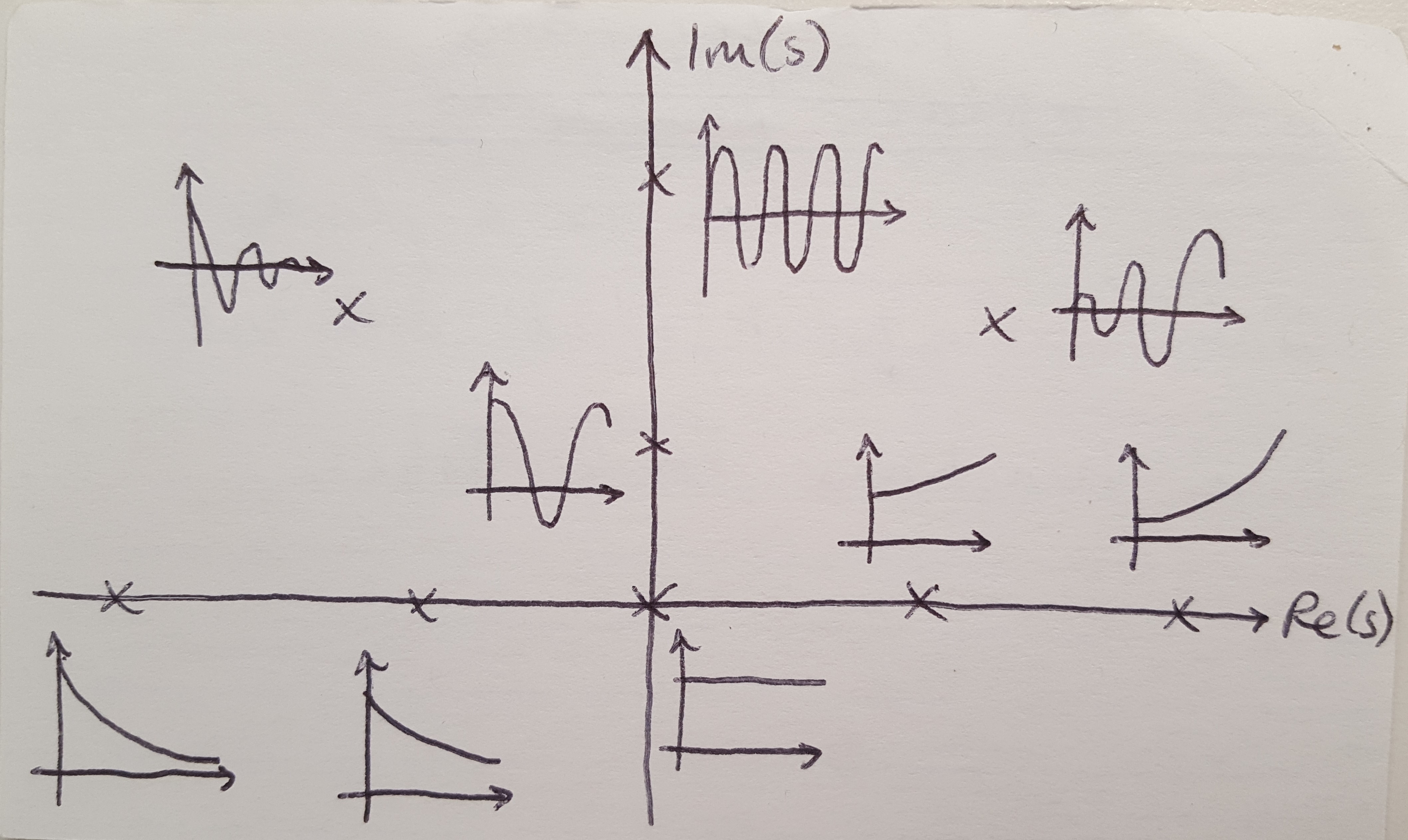
Figure 1

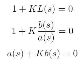
(2) The root locus plots the all the points that are solutions of the closed loop transfer function. We can write the CL TF equation in 3 ways but they all mean the same thing:

(3) The root locus contains all the points where the phase of the open loop transfer function is 180 degrees. This last definition is harder for me to wrap my head around, but it will come in useful when we have to draw the root locus later on.

Given these descriptions of the root locus, hopefully you can see that it contains a lot of useful information. We will come back to this idea after we have drawn a root locus plot to show how we can pull this information from the diagram. For now, let’s try to draw one. As an example, let’s consider the closed loop transfer function:

There are 5 rules for drawing a root locus plot as defined in [1]. We will work through them sequentially to get the root locus plot:

(1) N branches start at the poles of L(s). M branches end on the zeros of L(s). For this transfer function, we can see that the poles and zeros are:

Poles: 0, -1, -10, where N = 3
Zeros: -2, where M = 1

Notice that this means that, although N = 3 branches will start at the poles of L(s), only M = 1 branch will terminate at a zero. The other 2 branches will go to infinity. This rule comes from looking at the minimum and maximum values of K in the equation a(s) + Kb(s) = 0. When K = 0, then a(s) must also be 0, and so a(s) takes on the values of the poles of L(s), because L(s) = b(s) / a(s). Therefore the root locus starts (when K = 0) at the poles of L(s). When K goes to infinity, then either b(s) = 0 (in which case the root locus arrives at the zeros of L(s)) or s must go to infinity (which is what happens to the branches of the root locus that do not terminate at the zeros). I have drawn the root locus showing the poles and zeros on the s-plane to get us started.

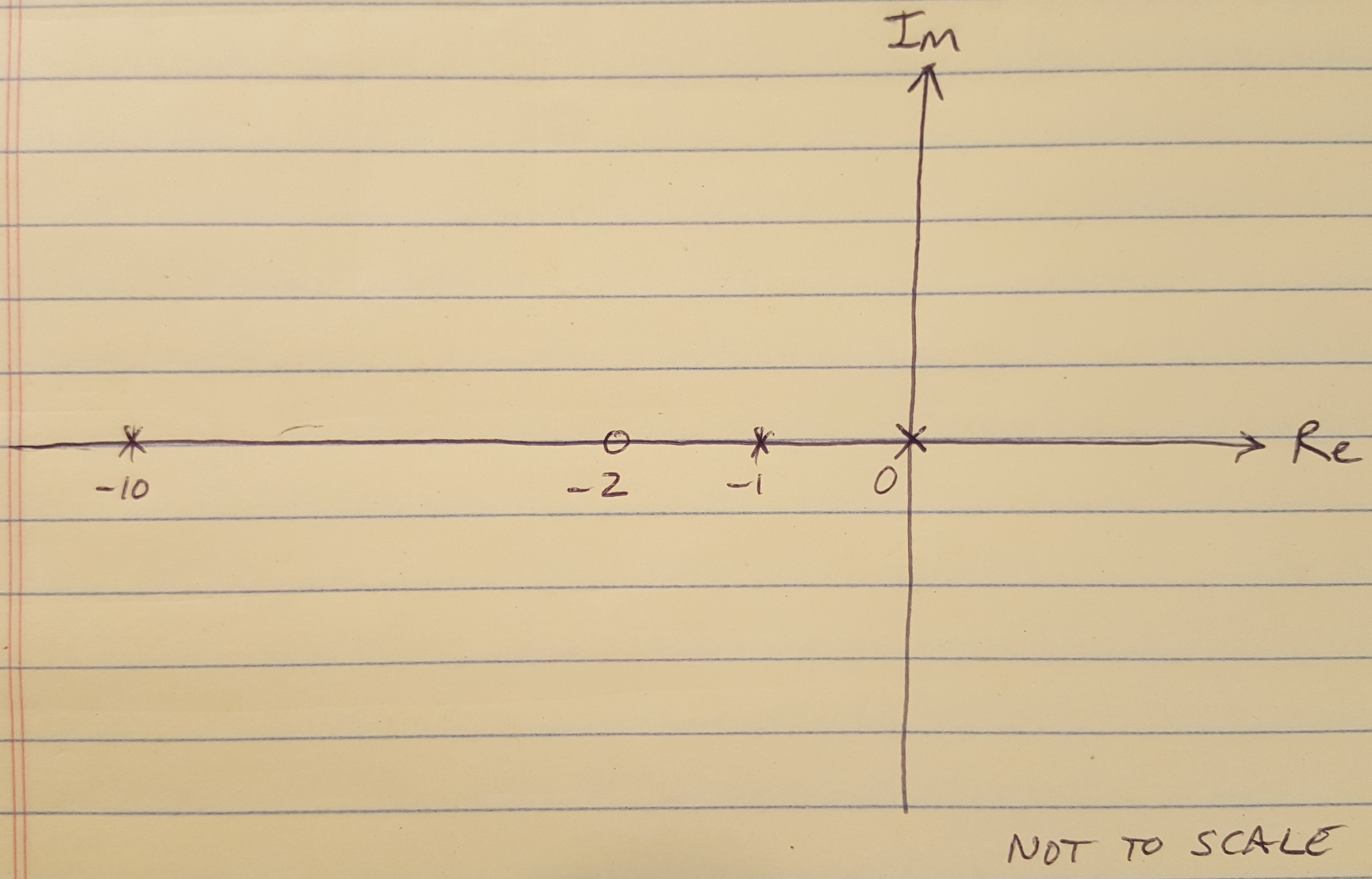
Figure 2

(2) Loci are on the Real axis to the left of an odd number of poles and zeros located on the Real axis. Although it is easy to implement this rule (I just did it below, take a look), it is a little more complicated to understand why it exists.

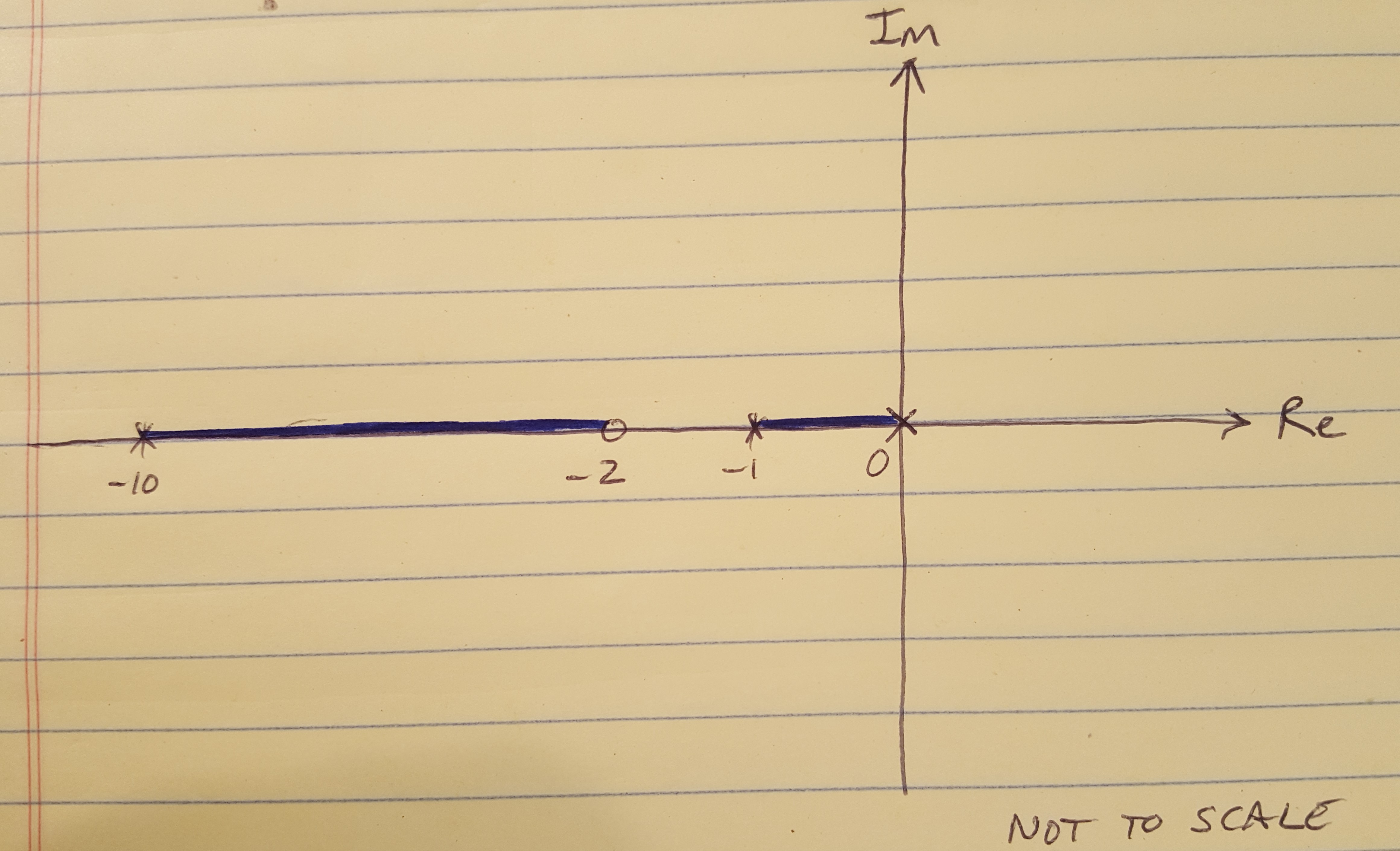
Figure 3

Do you remember the 3rd definition of the root locus above, that says that all the points on the root locus have a phase of 180 degrees? That requirement drives Rule 2 because if you consider some test point s_0 as shown below, in order for it to be on the root locus, the angles from the poles and zeros to that test point must sum to 180 degrees. We can see that this condition will be true any time we are to the left of an odd number of poles and zeros.

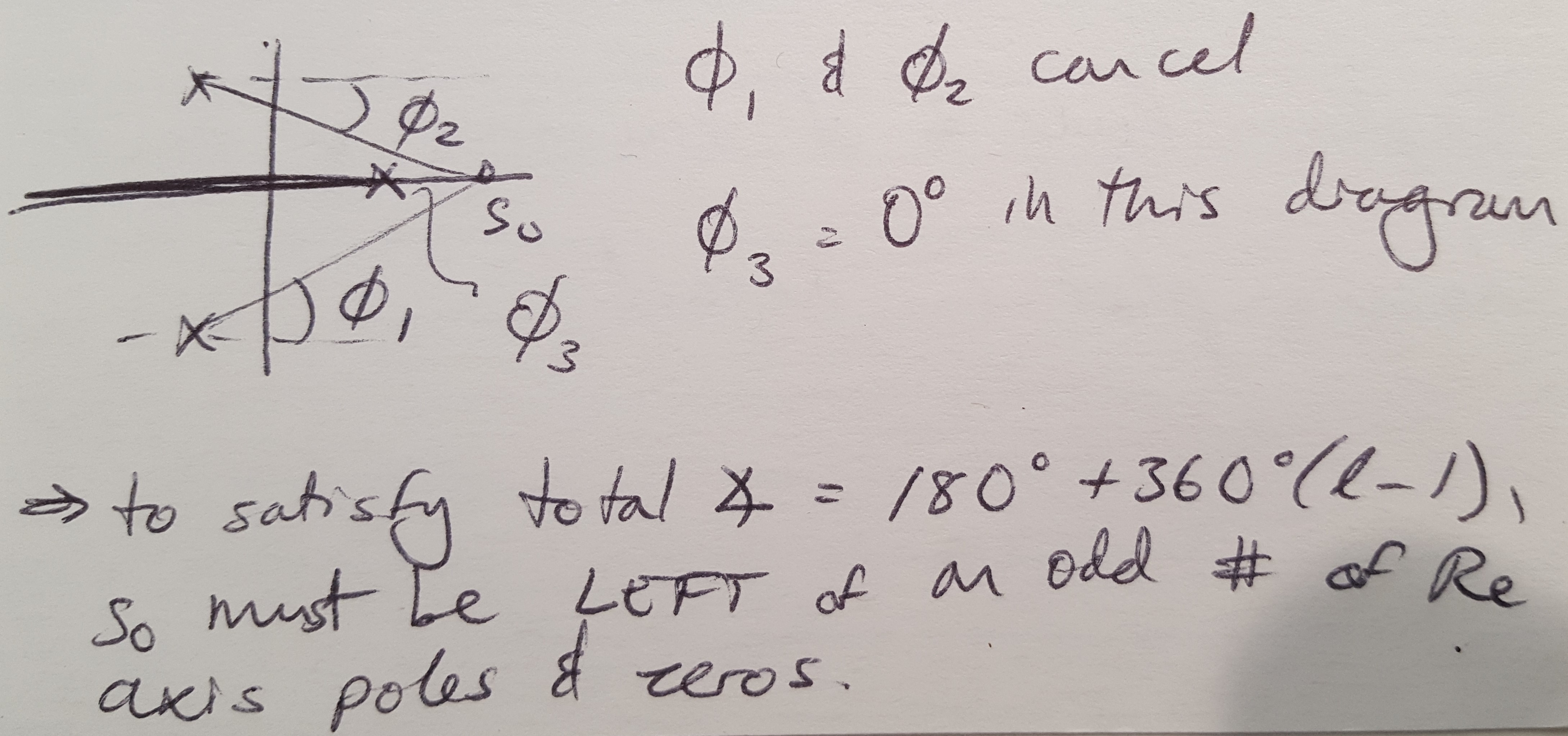
Figure 4

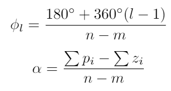
(3) For large values of K, the remaining N - M branches of the root locus are asymptotic to lines at specific angles, radiating from a center point s = a on the Real axis. We can calculate the angles and the center point using the equations below. For this example, I have calculated that there is an asymptote oriented at 90 degrees which originates at s = -4.5. You can see the asymptote drawn in red below.

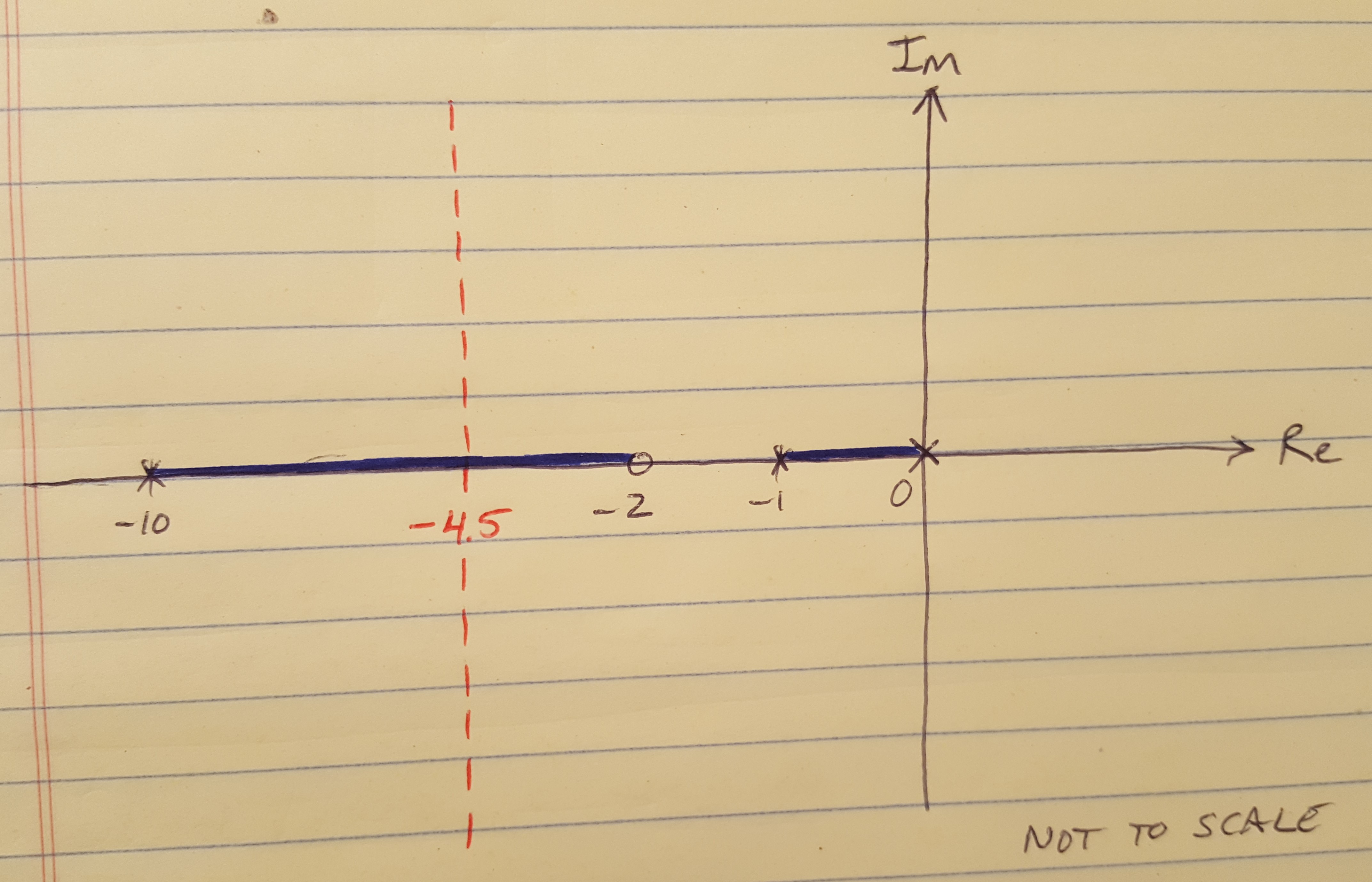
Figure 5

Okay, I know, this rule is confusing too, but we can figure out where it comes from. Let’s start with the angle of the asymptote. Again, this asymptote represents what happens when the gain, K, is very large. When the gain is large, we are on these N-M branches that are heading for infinity. Definition 3 from above is still in effect, so the sum of the angles from all the poles and zeros to our position on the asymptote must still be equal to 180 degrees. And when we are on the root locus but NOT on the Real axis, we are on all the asymptote branches simultaneously. That’s why the SUM of the N-M angles from the poles and zeros to our current locations must be equal to 180 degrees.

How about the equation for the center point? Well, if you imagine that we are a long way from the Real axis, somewhere on the asymptote, then you can imagine that all the poles and zeros of the system look as though they are clustered together. We can approximate the root locus equation as:

In this case, alpha is the point on the Real axis where all the poles and zeros appear to be clustered. The equation for alpha is found using some polynomial manipulation that I don’t want to describe in detail here, but you can read about it in [1].

(4) Angles of departure (branch leaving a pole) and angles of arrival (branch terminating at a zero) can be calculated. The equations for departure and arrival angles are:

Notice that they are for poles and zeros of multiplicity q. This means that we may have multiple poles and zeros stacked on top of each other. If that is the case, divide the answer by q (the number of stacked poles or zeros) to get the true arrival/departure angle. For this problem, we do not necessarily need to calculate these angles directly because we know that the branches depart from the poles along the Real axis using Rule 2.

(5) The locus can have multiple roots of multiplicity q, and the branches of the root locus will approach these q roots at angles as calculated in the equation below. This rule is for cases where multiple branches are approaching the Real axis and we want to find the angle at which they should intercept the Real axis. Again in this example, we don’t have this situation but it does come in handy for certain systems.

Okay, we are now done drawing our first root locus plot. In my next post, I will talk about how we can use this plot to pick a gain to meet our design requirements.

References

[1] Franklin, G., Powell, J.D., Emami-Naeini, A. Feedback Control of Dynamic Systems, 6th ed. Pearson. 2009.