In this post I am going to cover a new (to me) machine learning algorithm called support vector machines. Support vector machines (SVMs) are another form of supervised learning that can be used for classification and to perform regression* [1]. In this post we will start by learning the cost function for SVMs, then we’ll discuss why they are also called “large margin classifiers”, we will introduce kernels, and then we’ll finish with a discussion of how to choose the parameters for SVMs and when to use SVMs or logistic regression [3]. Let’s go!

SVM Cost Function

We’ll start by revisiting the cost function for logistic regression and tweak it to find the cost function for SVMs [3]. If you recall, logistic regression uses the sigmoid function as the activation function [3]. With SVMs, we replace the sigmoid function with two straight lines as shown in Figure 1 below [3]. We will just call this new function “cost-SVM” for now. Notice that if you want to predict y = 1 (and therefore you want the cost-SVM = 0), then you need theta’ * x to be greater than 1 [3]. Likewise, if you want y = 0 (and the cost-SVM = 0) then you want theta’ * x to be less than -1 [3]. This is different from logistic regression, where you just needed theta’ * x to be positive or negative to get a correct hypothesis [3].

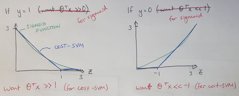
Figure 1 - adapted from [3]

We will also rearrange the position of the regularization parameter so that it is in front of the first term, not the second term, as in logistic regression [3]. To get some intuition for this, remember that the first term in the cost function is measuring the error in the prediction, and the second term is trying to minimize the size of the parameters, theta [3]. The regularization parameter allows us to tell the cost function how much to weight each of these priorities [3]. Moving the regularization parameter to be in front of the error measurement instead of the minimization of theta is not complicated, and results in the following expression for the cost function [3]:

Equation 1

To be honest, I am not sure why we want to rearrange the regularization term so that it is now in front of the error measurement (we call the regularization term C in the cost function for SVMs) but remember that C is the inverse of lambda [3]:

Equation 2

Remember how we pointed out in Figure 1 that we need theta’ * x to be greater than or equal to 1 to get a prediction of y = 1? This is part of the reason why we call SVMs “large margin classifiers” [3]. They are more robust than logistic regression classifiers because they need theta’ * x to pass some threshold before they make a prediction [3]. Another way to think about this is to look at the decision boundary separating two linearly separable sets of training samples, as shown in Figure 2 below [3]. The SVM is going to pick a decision boundary that maximizes the margin (that is, the distance) between the boundary and any of the training samples [3].** In the next section we will build on this intuition with a discussion of vectors.

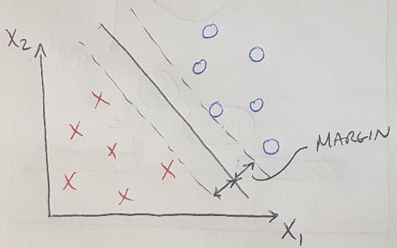
Figure 2 - adapted from [3]

Why SVMs are Large Margin Classifiers

If you recall from mathematics, the inner product of two vectors can be written in terms of the projection of one vector onto another and the magnitude of the first vector [3]. That is [3]:

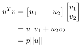
Equation 3

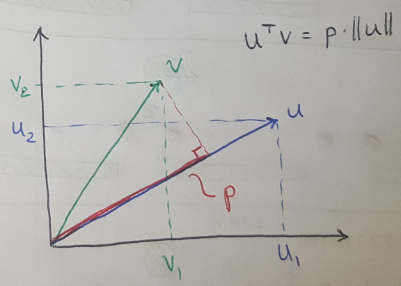
Figure 3 - adapted from [3]

We can also illustrate this idea as shown in Figure 3. We will use this fact to understand how the SVM is maximizing the margin on the decision boundary. Namely, let’s consider the situation where we have to minimize the size of the parameters, theta, in the cost function, because we have successfully made a prediction that y = 1 or y = 0 and that has set the first term in the cost function to 0 [3]. This can also be written as [3]:

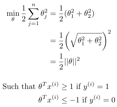
Equation 4

Note that we can also write the conditions on the optimization of the cost function to be in terms of the projection of x onto theta, and the norm of theta - as described in Equation 3 [3]. This would mean that we could now write our cost function as follows [3]:

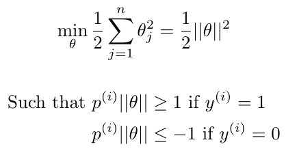
Equation 5

Now let’s consider two ways to draw our decision boundary through our training samples, as shown in Figure 4. In the left-hand image, our decision boundary has not done a good job of maximizing the margin between the boundary and the training samples. Let’s discuss the mathematical explanation for what is happening here. We know that the vector representing theta is always perpendicular to the training boundary, and the vector is shown below in Figure 4 [3]. The projections of each of the training samples onto the theta vector are also shown - in the image on the left, these projections are quite small [3]. That means that, in order to meet the conditions on our optimization (as described in Equation 5), we would need to choose very large values of theta [3]. But we can’t do that because then our cost function would return a very high value [3]! So what to do?

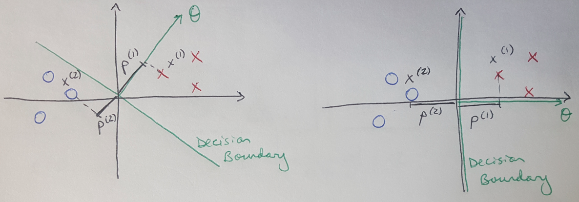
Figure 4 - adapted from [3]

Well, what happens if we place the decision boundary as shown in the right-hand image in Figure 4? Now we can see that the projections of the training samples onto the theta vector are much larger in length, and so we can make the norm of theta correspondingly smaller [3]. Now we have met our optimization constraints and minimized theta as much as possible [3]. This is what the SVM is doing.

Kernels Aren’t Just for Popcorn

Now let’s introduce the idea of a kernel into this discussion. The term “kernel” has multiple meanings***, but in this context it refers to a class of functions which are used in pattern analysis algorithms (also called kernel methods) [5]. Kernels are popular because they are computationally efficient [5]. They are used in SVMs but they are also used in Gaussian processes, principal component analysis, and other tools [5]. How do we use them in SVMs?

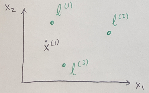
Figure 5 - adapted from [3]

Consider a situation where you need a nonlinear decision boundary to classify your training samples [3]. We can use kernels to specify the boundary instead of a complex polynomial [3]. Let’s imagine that we picked three landmarks as shown in Figure 5, and that we wanted to compute the similarity of a training sample, x, to each of these landmarks, l [3]. The function we use to compute the similarity is a kernel, and the most commonly used kernel for SVMs is a Gaussian kernel, which can be defined as follows [3]:

Equation 6

Each kernel will calculate how close the training sample is to a particular landmark, and return a value of 1 if the sample is close, and a 0 if the sample is far from the landmark [3]. Notice that there is a value of sigma in the expression for a Gaussian kernel [3]. The value of sigma determines how quickly the chance of the kernel returning a value of 1 falls away - that is, a larger sigma makes the kernel function fall away slowly, and a small sigma makes the kernel function fall away quickly [3]. This is illustrated in Figure 6 below [3].

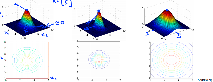
Figure 6 - Source [3]

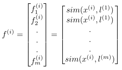
But how do I choose all of my landmarks? We will just set our landmarks equal to our training samples, so for every training sample, we will compute how close it is to all of the others [3]. We can write this as a feature vector [3]:

Equation 7

Then we would just replace the feature vector in our hypothesis as follows [3]:

Equation 8

Notice that when you are using kernels, you will want to perform feature scaling before you use them because otherwise the features that have larger numeric magnitudes will dominate the computation of the cost [3].

Choosing Parameters and Dealing with Bias/Variance in SVMs

Typically you can implement an SVM using standard libraries in different scripting languages, but you will typically need to pick some values yourself including the regularization parameter, C and the value for sigma [3]. Here’s how your choice of C will affect your bias and variance [3]:

Big C: Low bias, high variance (tends to overfit)
Small C: High bias, low variance (tends to underfit)

And your choice of sigma will also affect your bias and variance [3]:

Big sigma: Features vary more smoothly, high bias, low variance
Small sigma: Features vary more abruptly, low bias, high variance

Notice that you can also choose different kernels to use in your SVM, but no matter which function you choose, it must satisfy Mercer’s theorem, which constrains the kernel so that it can be optimized using most standard optimization packages [3].

When should we use SVMs over logistic regression? We can think about the choice in terms of the number of features, n, and the number of training samples that we have, m [3]:

(1) If n is large compared to m: Use logistic regression (or SVMs without a kernel (aka with a linear kernel)). In this case there is relatively little data available so you will not be able to effectively train a complex decision boundary, and a relatively simple logistic regression algorithm will perform better [3].

(2) If n is small and m is of medium size: Use SVMs with Gaussian kernels.

(3) If n is small and m is large: create or add more features (n) and then use logistic regression or SVM without a kernel, because it will be too computationally expensive to use SVMs with Gaussian kernels [3].

I think that is about it for SVMs, I hope this was useful.

Footnotes:

*Regression analysis is a set of statistical processes that can be used to find the relationship between a dependent variable and a group of independent variables [2]. Linear regression is a common example, where you try to fit a line to a set of data to show the relationship between x (the dependent variable) and y (the independent variable) [2].

**Just as a side note, the choice of regularization parameter, C, will affect how much this decision boundary moves when outliers appear in the datasets [3]. Large values of C will force the decision boundary to move a lot; smaller values of C will only force the decision boundary a little bit, if at all [3].

***For example, in operating system architecture, a kernel is a program at the center of a computer’s operating system which has complete control over every part of the system [4].

References:

[1] Wikipedia. “Support vector machine.” https://en.wikipedia.org/wiki/Support_vector_machine Visited 16 May 2020.

[2] Wikipedia. “Regression analysis.” https://en.wikipedia.org/wiki/Regression_analysis Visited 16 May 2020.

[3] Ng, A. Machine Learning course, week 7 lecture notes on support vector machines. Coursera. https://www.coursera.org/learn/machine-learning/home/week/7 Visited 16 May 2020.

[4] Wikipedia. “Kernel (operating system).” https://en.wikipedia.org/wiki/Kernel_(operating_system) Visited 16 May 2020.

[5] Wikipedia. “Kernel method.” https://en.wikipedia.org/wiki/Kernel_method Visited 16 May 2020.