Recently I have been interested in constructing scene graphs directly from raw image data for a research project. Scene graphs are a representation of the objects in an image, as well as their relationships [1]. Typically, a scene graph represents the objects as nodes and joins these objects together using edges and nodes that represent specific types of relationships [1]. It can be useful to construct graphs from images so that we can use the graph information as part of a larger AI solution that operates on graphs. In the post we are going to focus on a particular method for deriving scene graphs from images as proposed by Prof. Fei-Fei Li’s group at Stanford in “Scene Graph Generation by Iterative Message Passing” by Xu et al. [1].

Overview

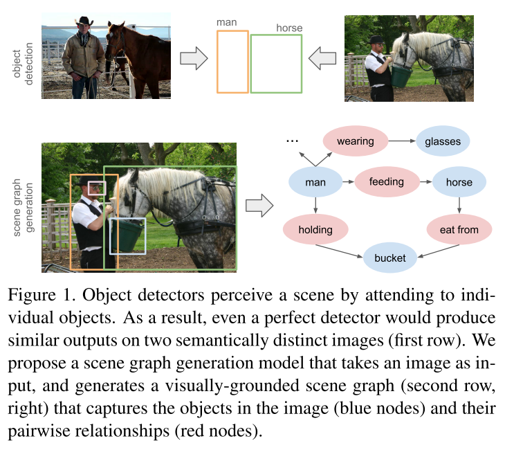
Figure 1 - Source: [1]

In this paper, our objective is to take as input a single image, and to return as output a scene graph that completely describes the objects in the image and their relationships [1]. This concept is illustrated in Figure 1. The proposed solution uses several concepts from artificial intelligence, computer vision and Bayesian probability. Xu et al. use a standard recursive neural network (RNN) to infer the structure of the graph, and it uses message passing to improve its predictions of the scene graph over multiple iterations [1]. They also use a joint inference model to use the image context to improve predictions as well [1]. An overview of the model architecture is shown in Figure 2. The entire solution is an end-to-end model*1 which returns a scene graph with object categories, the bounding boxes of the objects found in the image, and the relationships between pairs of objects [1].

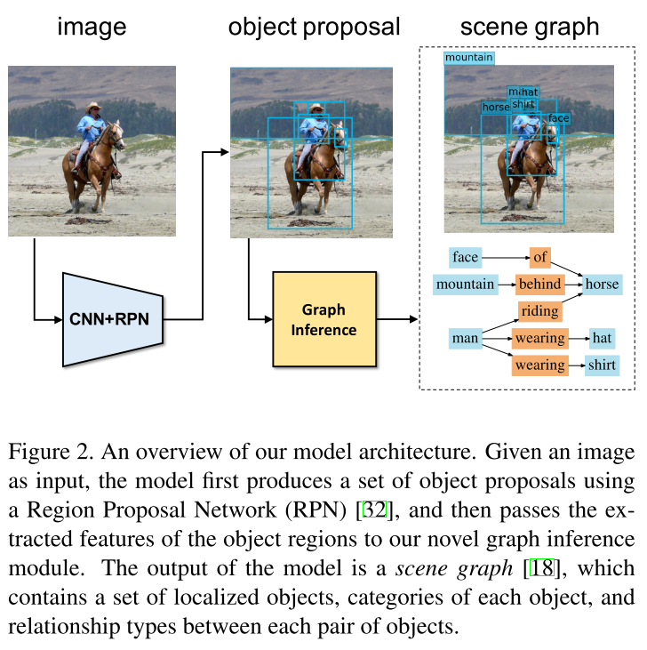
Figure 2 - Source: [1]

Introducing Bipartite Graphs, GRUs and Message Passing

The scene graph that is built during this process can be described as bipartite, which means that the nodes in the graph can be divided into two distinct sets, and every edge joins a node from each set [3]. In this context, the scene graph is bipartite because it contains two types of nodes: nodes that represent objects (horse, mountain, face) and nodes that represent relationships (of, riding, wearing) [1].

Xu et al. explain that their approach to performing dense graph inference is inspired by work by Zheng et al. [4] which uses RNNs to complete the inference [1]. Let me briefly try to explain what I mean by dense graph inference: first, we are assuming that most of these scene graphs are going to be dense - that is, that there will be many connections, or relationships, between objects in the graph. Secondly, we are trying to infer what the structure and contents of the scene graph should be using probability - we will go into more detail on this point in a subsequent section.

The point that Xu et al. are trying to make here is that while the previous work by Zheng et al. also used RNNs, the prior work used custom RNN layers, while this work by Xu et al. chose to use a generic RNN layer, called a gated recurrent unit (GRU), instead [1]. The advantage, they argue, is that Xu et al.’s architecture is more flexible and general-purpose than the earlier work by Zheng et al. [1].

Let’s briefly review what a RNN and a GRU are. A recurrent neural network is a type of neural network that is typically used to process sequential data [5]. There are different types of RNNs, and one type in particular is the GRU, developed by Cho et al. in 2014 [5]. The GRU is a unit that takes in input at a given time step, and combines it with knowledge derived from prior time steps (called the hidden state) and updates that hidden state at the current time point [5]. A GIF prepared by Raimi Karim is shown below, and he recommends reading this post by Michael Phi to learn more about RNNs if you’re interested.

Figure 3 - Source: [5]

The tricky part to understand here is how the GRUs are used to build the scene graph and perform message passing over the graph. Xu et al. explain that each node and edge in the scene graph store their “internal states” inside a corresponding GRU unit [1]. So there is one GRU unit per node and per edge in the scene graph. We also note that all the node GRUs share the same set of weights, and similarly all the edge GRUs also share the same set of weights (but a different set from the node GRUs) [1]. Information is shared by passing messages between GRUs (more on that later) [1].

The bipartite graph structure is going to come into play in this message-passing process, too. Since, by definition, our bipartite scene graph will only have edges connecting object nodes to relationship nodes (and vice versa), we know that there is no message passing inside the set of object nodes or the set of relationship nodes [1]. This means that we can think of the subset of object nodes as the dual graph*2 of the subset of relationship nodes [1].

In a slightly confusing use of vocabulary, Xu et al. also present the message passing problem as a “primal-dual graph” structure, where the primal graph represents the pathways for messages to move from edge GRUs to node GRUs, and the dual graph represents the pathways for message passing from node GRUs to edge GRUs [1]. I’m confused because I think the “primal-dual” terminology is often used to mean other things than what is happening here, but maybe I just don’t have enough of a graph theory background to really grasp this. Either way, this concept is illustrated in more detail in Figure 5.

Now that we have introduced the basic architecture used by Xu et al., let’s dive deeper into the mathematics of the graph inference problem.

The Graph Inference Problem

In this section we are going to see how we take the input image, apply bounding boxes, and generate the object class and relationship type for each object and pair of objects, respectively. To obtain preliminary bounding boxes, the authors use the Region Proposal Network to get a set of proposed bounding boxes as a starting point for the inference model [1].

The authors take in the proposed bounding boxes and infer object classes for each identified object. They also find offsets for the proposed bounding boxes to refine the size and location of each box. Lastly, they identify relationships between each pair of objects. If we define the set of object classes as C and the set of relationship types as R, then we can write [1]:

Equation 1

Ultimately, our goal is to find an optimal set of variables, x*, which maximizes this probability [1]:

Equation 2

In the next section, we will see how we can approximate this inference using GRUs to perform iterative message passing [1].

Approximating Graph Inference using GRUs and Message Passing

Xu et al. use an approach called “mean field” to approximate the graph inference we described in Equation 2 above [1]. I am not sure what “mean field” is, but we can discuss the mechanics of this approach regardless. First, we define the probability of each variable, x, as [1]:

Equation 3

The nodes and edges each have some hidden states that are computed by the corresponding GRUs [1]. Together all of these computations form an expression for the “mean field distribution” which can be written as [1]:

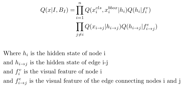
Equation 4

Please note that the term visual feature refers to the proposed bounding box in the case of individual nodes, and it refers to the union box that fits over the bounding boxes for the nodes i and j in the case of individual edges [1].

Earlier we discussed the concept of a primal-dual graph structure, where the primal graph describes how messages flow from edges to nodes, and the dual graph describes the flow of information from nodes to edges. Xu et al. point out that by identifying this unique structure, we can reduce the number of computations that we have to perform as compared to processing all connections that are present on a generic dense graph [1].

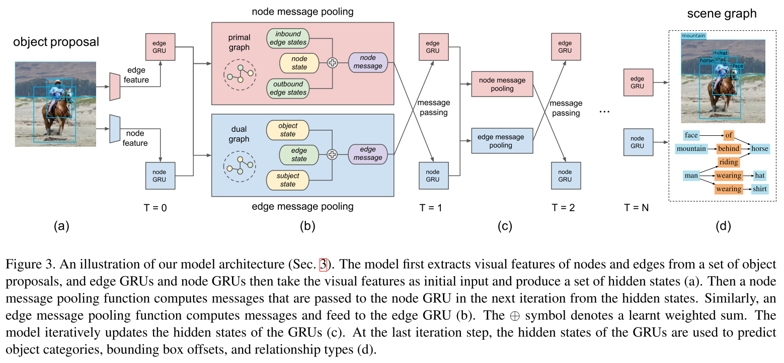
Figure 5 - Source: [1]

Since every node GRU could be receiving inputs over multiple edges (see Figure 5), we need to find a way to pool or aggregate all the incoming messages [1]. Xu et al. use a weighted function so that they can learn weights for each individual incoming message - this helps the model learn which information is more valuable in computing the graph inference [1]. We can write expressions for the messages that are pooled for the nodes and edges as follows [1]:

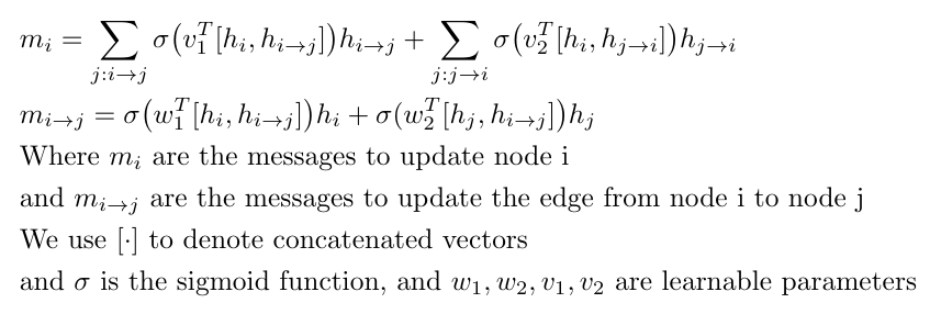
Equation 5

This concludes the details of the theory behind scene graph generation as presented in Xu et al. Please do consider reading the paper in its entirety - there is much more information available than I covered here.

Footnotes:

*1 The expression “end-to-end” just means that the model takes in some input and returns the thing we are looking for, without any post processing [2]. In other words, it is the complete solution [2].

*2 A dual graph is a complementary graph that places a node at every face of the graph it is complementing [6]. Consider Figure 4 as an illustration of this concept.

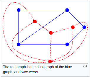
Figure 4 - Source: [6]

References:

[1] D. Xu, Y. Zhu, C. B. Choy, and L. Fei-Fei, “Scene Graph Generation by Iterative Message Passing.” https://arxiv.org/abs/1701.02426 Visited 8 Nov 2020.

[2] “What does end to end mean in deep learning methods?” Quora. https://www.quora.com/What-does-end-to-end-mean-in-deep-learning-methods Visited 8 Nov 2020.

[3] “Bipartite graphs.” Wikipedia. https://en.wikipedia.org/wiki/Bipartite_graph Visited 8 Nov 2020.

[4] S. Zheng, S. Jayasumana, B. Romera-Paredes, V. Vineet, Z. Su, D. Du, C. Huang, and P. Torr. Conditional random fields as recurrent neural networks. In International Conference on Computer Vision (ICCV), 2015. https://arxiv.org/abs/1502.03240 Visited 8 Nov 2020.

[5] Karim, R. “Animated RNN, LSTM and GRU.” 14 Dec 2018. Towards Data Science on Medium. https://towardsdatascience.com/animated-rnn-lstm-and-gru-ef124d06cf45 Visited 8 Nov 2020.

[6] “Dual graph.” Wikipedia. https://en.wikipedia.org/wiki/Dual_graph Visited 8 Nov 2020.