In this post we are going to cover a couple of fundamental algorithms, including a common search algorithm known as binary search, as well as two sorting methods, merge sort and quick sort [1]. For each algorithm, we will talk through how they work and some details on runtime. If you are looking for some example code, please see my implementations for binary sort, taken from [2], merge sort taken from [3] and quick sort taken from [4].

Binary Search

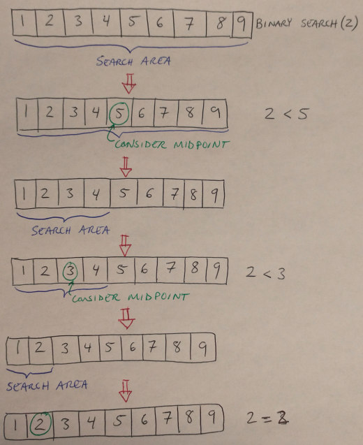
In binary search, we assume that we are starting with a sorted array, and that we are looking for a particular item within that array [1]. We choose the midpoint of the array, and compare it to the value we are searching for [1]. If the midpoint is smaller than the value, then we know to look to the right (i.e. to the larger entries); if the midpoint is larger than the value, then we look to the left (i.e. to the smaller entities) [1]. This effectively cuts the array in half, and then we repeat the process: we look at the midpoint, and based on how it compares to the value we are searching for, we either go left or right. We repeat this process until we find our desired value.

Figure 1

The runtime of binary search is the base-2 logarithm of the number of elements in the array, log(n), because every iteration of the algorithm halves the number of elements we look through [2]. Binary search uses the divide-and-conquer technique, which breaks up a problem into many identical sub-problems [2]. (The quick sort and merge sort algorithms are also an example of divide-and-conquer, as we’ll see in a minute [2].) This runtime is pretty fast, but it is not the fastest search algorithm out there [2]. However, it balances time and memory requirements better than some other algorithms that are faster but more memory intensive [2].

Merge Sort

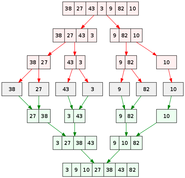
Merge sort can be used to sort arrays using a divide-and-conquer method. It works by taking an array and dividing it in half [1]. Each half is sorted independently, and then the two halves are merged together (in correct order) [1]. This is a recursive approach, so the same process of dividing the array in half and sorting the halves is applied to each half of the original array [1,3]. This is repeated until the algorithm reaches the base case, which is sorting two adjacent elements in the array [1]. Once the pairs are sorted, they are merged again. The merge process must check that the two pairs are merged correctly in order of their value, so it steps through the values in the two pairs and assigns the four values to the base array in order of their size [3]. The algorithm is illustrated graphically in Figure 2.

Figure 2 - Source [5]

The runtime of merge sort is O(n log(n)) for both the average and worst cases. The log(n) comes from the fact that each step in the recursion divides the array in half, and the n component comes from the linear time required to merge the two half-arrays together [3].

Quick Sort

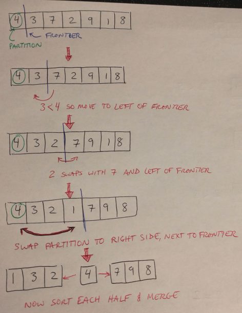
Quick sort is also used to sort an array, and uses a divide-and-conquer approach. It can be implemented both recursively (because it is a divide-and-conquer approach) and iteratively, although generally the recursive approach is preferred [4]. The quick sort method chooses a random element in the array to serve as the pivot [1]. The array is partitioned using a series of swap operations so that at the end of the partitioning process, all the numbers that are smaller than the pivot are to its left [1]. Then the process is repeated with the left and right halves of the array until all the elements are sorted [1]. This process is nicely illustrated on Edpresso’s website if you would like to see an animation [4]. It is also illustrated in Figure 3.

Figure 3

The runtime for quick sort, in the worst case, is n^2, because there is no guarantee that the algorithm will choose the median element as the partition [1]. If a number far from the median is chosen (say the minimum or maximum), then the partitioning process could take up to n^2 time. However, if a value close to the median is chosen, then the runtime is closer to O(n log(n)), similar to merge sort [1].

Alright, that concludes this post on some basic searching and sorting algorithms. I will probably not be posting again on basic coding interview concepts for a while - I’m going to focus on solving problems in [1]. If you, too, are interested in practicing your coding problems, you can find a set of Python solutions to the problems in [1] here. Good luck!

References:

[1] Laakmann McDowell, G. Cracking the Coding Interview, 6th edition. 2016. CareerCup, LLC.

[2] Zaczynski, B. “How to Do a Binary Search in Python.” Real Python. 16 Mar 2020. https://realpython.com/binary-search-python/ Visited 28 Jan 2021.

[3] “Merge Sort.” GeeksforGeeks. 02 Feb 2021. https://www.geeksforgeeks.org/merge-sort/ Visited 02 Feb 2021.

[4] “How to implement QuickSort in Python.” Edpresso. https://www.educative.io/edpresso/how-to-implement-quicksort-in-python Visited 02 Feb 2021.

[5] VineetKumar. Merge sort algorithm diagram.svg. Wikipedia. 18 Sept 2007. https://en.wikipedia.org/wiki/File:Merge_sort_algorithm_diagram.svg#file Visited 02 Feb 2021.