It is Day 2 of my (entirely made-up) Silver Challenge! Today I want to highlight what I learned about the Bellman Equation, which I have also struggled to understand in the past. The Bellman Equation (in various forms) is used to recursively solve for the value function in a reinforcement learning problem [1]. We saw the Bellman Equation used to solve Markov Reward Processes (MRPs) and Markov Decision Processes (MDPs) [1]. In both cases, the Bellman Equation recursively decomposes the value function into two parts: (1) the immediate reward and (2) the discounted value of the successor state [1]. Silver further emphasizes that the key idea of the Bellman Equation is that it allows you to solve for the value function [1].

Let’s take a closer look at this idea - we will start with getting some intuition for the Bellman Equation for MRPs, then the extension of the Bellman Expectation Equation for MDPs, and concluding with the Bellman Optimality Equation [1].

Bellman Equation for MRPs

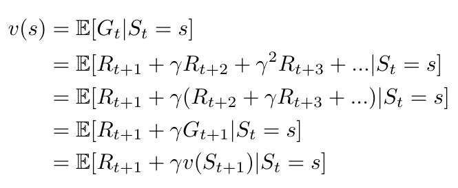
In the introduction we explained that the Bellman Equation allows us to solve the value function by decomposing it into two parts [1]. Let’s see how that works mathematically for Markov Reward Processes (in an MRP, we do not yet consider making decisions and generating actions) [1]:

Equation 1

Now I can solve the Bellman Equation with a closed form solution by following a couple of steps. First, we can rewrite the result of Equation 1 as a function of the state transition probability matrix (thereby removing the expectation) [1]:

Equation 2

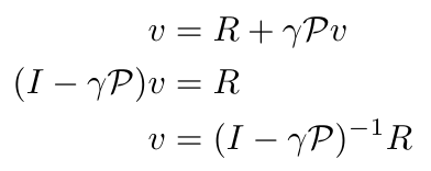
Then I can convert this expression to matrix form, and solve it using the matrix inverse function [1]:

Equation 3

Notice that the complexity of computing a matrix inverse is O(n^3) so this approach will not work for large states [1]. Instead, we can solve this problem using iterative solutions which we will see in subsequent lectures [1].

Bellman Expectation Equation for MDPs

An MDP is different from an MRP because it now takes the actions of the agent, and the corresponding policy that governs the agent’s behavior, into account [1]. However, despite this difference the key idea to the Bellman Equation still holds true: we are still using it to recursively solve for the value function by decomposing it into two parts [1]. The difference is that now we are applying the Bellman Expectation Equation to two value functions: the state-value function and the action-value function [1]. We can write these as follows [1]:

Equation 4

And again I can rewrite Equation 4 to generate a matrix form of the Bellman Expectation Equation [1]. First I write Equation 4 as a function of the policy [1]:

Equation 5

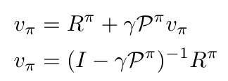
Then I write the matrix version of Equation 5 (in this example I will just write it out for the state-value function, v), and solve again using matrix inversion [1]:

Equation 6

As before, this gets difficult to solve for large systems and so we will look at other ways to solve this expression in subsequent lectures.

Bellman Optimality Equation

Finally, we don’t just want to find a value function, we want to find the optimal value function [1]. Remember, our ultimate goal in RL is to find the optimal policy, and in order to find the optimal policy, we need to optimize both the state-value and action-value functions [1]. (Actually, all we really need to know is the optimal action-value function, because then if we always choose the action that maximizes that function, we have found the optimal policy [1].) We can use the Bellman Optimality Equation to optimize both value functions [1]. For both value functions, we average over the state transition probabilities and maximize over the possible actions [1]. Mathematically, this looks like [1]:

Equation 7

It is impossible to find a closed form solution for the Bellman Optimality Equation because it is nonlinear [1]. (Specifically, the max function makes the equations nonlinear [1].) So we will need to, again, use iterative solution methods including value iteration, policy iteration, Q-learning and SARSA to solve these equations instead [1].

References:

[1] Silver, D. “RL Course by David Silver - Lecture 2: Markov Decision Process.” YouTube. 13 May 2015. https://www.youtube.com/watch?v=lfHX2hHRMVQ&list=PLzuuYNsE1EZAXYR4FJ75jcJseBmo4KQ9-&index=2 Visited 07 Aug 2020.