Things are getting exciting on the Silver Challenge! Today we started learning about model-free control, and various on-policy and off-policy approaches to solving the problem. We ended the lecture with an introduction to Q-learning, which I want to recap here because it seems to be a very important algorithm to know in the world of RL.

Q-learning is a method of performing off-policy control [1]. As we have discussed before, off-policy approaches involve two policies: the target policy, pi, and the behavior policy, mu [1]. In off-policy, the goal of having these two policies is that we want the target policy to become the optimal policy, while the behavior policy gives us the ability to fully explore the state space to ensure that we find the globally optimal policy [1]. Q-learning is a powerful approach because it allows us to improve both the target and behavior policies during the learning process [1]. Let’s look at this in a little more detail.

The target policy is optimized using a purely greedy method with respect to the action-value function, Q(s,a’) [1]. Mathematically, we can write [1]:

Equation 1

Similarly, the behavior policy, mu, is optimized using an epsilon-greedy method with respect to Q(s,a), which means that the behavior policy is allowed to explore the state space [1].

Notice that I said that the target policy is computed with respect to a’, not a. Why do we make that distinction? It is because the Q-learning method is allowing us to consider the relative value of two different actions [1]. In other words, the Q-learning method is performing updates by following actions, a, dictated by the behavior policy, but at every step it is also considering what reward we might have earned if we had followed the target policy instead, and chosen action a’ [1]. By considering the merit of following the target policy as well as the behavior policy, we can update the Q-function, Q(s,a), towards the target policy [1]. This ensures that the behavior policy does not pull us too far away from what we think is going to be the optimal policy [1].

Let me explain the merit of following the behavior policy’s recommended action, a, as well as the alternative action recommended by the target policy, a’, using math. The Q-learning target can be written, and simplified, as follows, where the text in black indicates values obtained from the behavior policy, and text in red indicates values obtained from the target policy [1]:

Equation 2

Equation 2 tells us that the Q-learning target is a combination of information from the behavior policy and the target policy. This Q-learning target is used to update the Q-function as follows [1]:

Equation 3

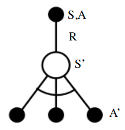
A nice image to represent the Q-learning algorithm another way is shown below in Figure 1.

Figure 1 - Source: [2]

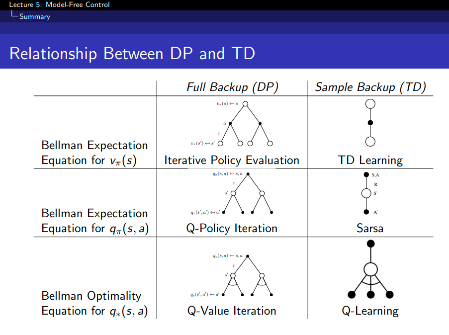
I also included a copy of the table that David Silver provided which summarizes the dynamic programming and sampling approaches to implementing various forms of the Bellman equation to solve problems of prediction and control in reinforcement learning, as shown in Figure 2.

Figure 2 - Source: [2]

References:

[1] Silver, D. “RL Course by David Silver - Lecture 5: Model Free Control.” YouTube. 13 May 2015. https://www.youtube.com/watch?v=0g4j2k_Ggc4&list=PLqYmG7hTraZDM-OYHWgPebj2MfCFzFObQ&index=5 Visited 10 Aug 2020.

[2] Silver, D. “Lecture 5: Model-Free Control.” https://www.davidsilver.uk/wp-content/uploads/2020/03/control.pdf Visited 10 Aug 2020.