Today is going to be a learning bonanza of topics related to machine learning (ML) and reinforcement learning (RL). I am working on a project that involves a lot of advanced ML/RL tools that I am trying to learn about very quickly. To that end, I have decided that today I am just going to write as many posts as possible on the topics that I need to understand. These posts may not be the most detailed essays I have ever written, but as always I will do my best to read several sources, cite them as appropriate, and only write about things I actually understand. Let’s go!

Basics of Variational Autoencoders

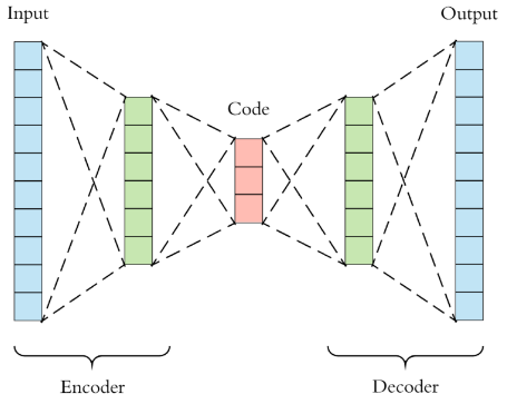
My project will use a special kind of neural network, called a variational autoencoder (VAE). Variational autoencoders are used to generate novel outputs by drawing from a collection of learned features that the network obtained from the training data [1]. As an example, we might use a VAE to generate scenery in video games - we train the neural network to understand what characteristics trees have, and then use the VAE to generate new images of trees that still look like trees [1]. Autoencoders are an entire class of neural networks that were originally designed as a form of data compression [1]. The objective of an autoencoder is to use a minimal number of nodes in the hidden layer to represent the input with sufficient resolution that it could be perfectly recreated by the output layer [1]*.

Figure 1 - Source [1]. Note that the red section in the middle (labeled “Code”) represents the latent space of the autoencoder.

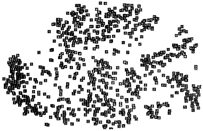
Variational autoencoders have 4 key components: an encoder, the latent space, a decoder and a loss function (see Figure 1) [3]. The encoder takes in the input data, X, and converts it to a set of values, F, that represent X [1,3]. We can call the set of values F the latent space [1]. The latent space is “latent” because it is hidden from the user [4]. The purpose of the latent space is to store all the necessary features of the model, so that the VAE can sample from points in the latent space and generate new outputs that have the same key characteristics as the input data [1,4]. The latent space is a compressed representation of just the key features of the training data, so it is useful in data compression algorithms (as we discussed above) because it has a smaller size than the training data itself - see Figure 2 for an illustration of the latent space [4,6]. Points in the latent space that are closer together are understood to be more similar to each other (for example, two adjacent points may be an pine tree and a Douglas fir tree - both types of evergreens) while points that are farther apart are more likely to be different (for example, a Douglas fir tree would probably be far from a palm tree in the latent space of trees) [4].

Figure 2 - Source [6]. A representation of the latent space of a neural network that is learning to classify the MNIST collection of handwritten numbers. Notice that all the images are grouped together by number, and numbers that look similar to each other are closer than those that are more distinct from one another.

Once the data has been compressed into the latent space, F, the decoder, a second neural network, is trained to take samples from the latent space and reconstruct the data, X, from that point in the latent space [1,3]. The entire VAE learns by trying to minimize a loss function, which is the typical expression for the mean squared error (MSE) between the input data, X, and the output data, X’ [1]. The output for each layer in the encoder NN can be written as [1]:

Equation 1

Where g is the activation function, theta represents the weights and b represents the bias terms [1]. The input data is X. We can also write the output for the decoder as [1]:

Equation 2

And therefore we can write the loss function for this neural network as [1]:

Equation 3

We try to balance the number of nodes in the encoder and decoder functions so that we have enough nodes to accurately compress and decompress the training data, but we don’t want to have so many nodes that the computation is inefficient and there’s no benefit to doing the data compression in the first place [1].

Probability and VAEs

In general, a standard autoencoder is trained on discrete data, so the latent space is also composed of a discrete set of points [1]. You can imagine that, unless you have trained the autoencoder on a huge dataset, there will be gaps in the latent space where the autoencoder has never seen a training example with exactly those features [1]. The latent space may also have trouble separating points that have features which are too similar - for example, if the autoencoder is learning to compress hand-written numbers, the latent space may have mixed up points for 0’s and 9’s because they look so similar [1]. This can make it difficult for the decoder in an autoencoder to accurately reconstruct data [1]. (Both of these phenomena can be observed in Figure 2.)

One way to address this problem is to change from representing the latent space as a discrete set of points to instead represent it as a probability distribution [1]. If we choose to represent the latent space as, for instance, a standard Gaussian distribution**, then we can randomly sample a point from anywhere inside that distribution and decode it [1]. This approach will not have any gaps because the Gaussian distribution is continuous. The general form of the probability density function is [5]:

Equation 4

Where mu is the mean, sigma^2 is the variance, and we can also denote this distribution as [5]:

Equation 5

Now that we have brought probability into the mix, we can revisit the mathematics behind the encoder, decoder and loss functions and rewrite the equations above from the probability perspective instead. For example, we can say that the encoder is going to learn to represent the latent space as a Gaussian probability density, and we can denote this as q(z given x) [3]. The function, q, is the Gaussian probability density, and it represents the probability that we get a certain value z_i given a certain input, x_i [3]. In other words, the encoder is learning the probability of z given x [1]. Similarly, the decoder is trying to do the opposite - it can be represented by a function p(x given z) and we can say that it is trying to learn the probability of x given z [3].

The loss function will still calculate the error between the decoder’s output and the desired output from the training data, and we will still use the loss function to do backpropagation over the entire VAE, calculate the derivatives for gradient descent and train the weights, theta [1,3]. I will stop the post here, however, because the details of how we calculate the loss function are very complicated, since we are now dealing with probability distributions and not simple discrete representations.

Footnotes:

*This can also be thought of as a form of principal component analysis [2], because the nodes in the hidden layer have activation functions that are directly and independently related to each of the input nodes.

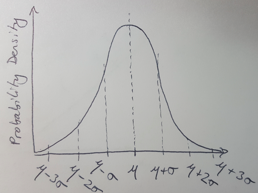
**A Gaussian distribution is a normal distribution of a real-valued random variable [5]. We use this probability distribution all the time in science because the Central Limit Theorem suggests that if we take many observations of a random variable and average them together, the distribution of the average will converge on a normal distribution as we take more and more samples [5]. Basically, a lot of things in nature look like Gaussian distributions so they are a good representation of a random variable that we don’t understand - like, for example, our VAE’s training data. The figure below is a reminder of what a Gaussian distribution looks like.

Figure 3 - The Gaussian (normal) distribution.

References:

[1] Stewart, M. “Comprehensive Introduction to Autoencoders.” 14 April, 2019. Medium: Towards Data Science. https://towardsdatascience.com/generating-images-with-autoencoders-77fd3a8dd368 Visited 24 March 2020.

[2] Wikipedia. “Principal component analysis.” https://en.wikipedia.org/wiki/Principal_component_analysis Visited 06 May 2020.

[3] Altosaar, J. “Tutorial - What is a variational autoencoder?” https://jaan.io/what-is-variational-autoencoder-vae-tutorial/ Visited 06 May 2020.

[4] Tiu, E. “Understanding Latent Space in Machine Learning.” 04 Feb 2020. https://towardsdatascience.com/understanding-latent-space-in-machine-learning-de5a7c687d8d Visited 06 May 2020.

[5] Wikipedia. “Normal distribution.” https://en.wikipedia.org/wiki/Normal_distribution Visited 06 May 2020.

[6] Despois, J. “Latent space visualization - Deep Learning bits #2.” Hackernoon. https://hackernoon.com/latent-space-visualization-deep-learning-bits-2-bd09a46920df Visited 06 May 2020.