This week I have been interested in reading papers about how to model time series data using unsupervised methods in machine learning. I will briefly summarize a couple of papers on the topic below.

Paper 1: VELC: A New Variational Auto Encoder Based Model for Time Series Anomaly Detection by Zhang et al.

This paper presents a method for finding anomalies in time series data using variational autoencoders. I did not know what anomaly detection really was until I read this paper - it is essentially the practice of looking for rare events in the data that are very different from the rest of the dataset, but are likely to be important, not random noise. Anomaly detection can be really difficult to do in a supervised fashion because the size of the anomaly class will generally be much smaller than the size of the “normal” class. But this paper proposes an unsupervised learning approach that side-steps that problem [1].

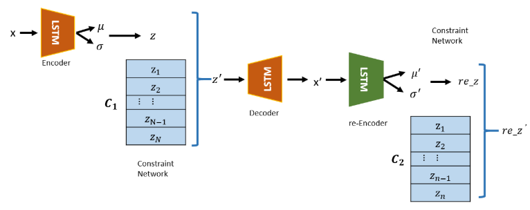
The authors introduce a VAE that has an additional re-Encoder and Latent Constraint network (VELC) that helps the model tell the difference between normal and anomalous data based on how well the model can reconstruct the input data. The basic idea here is that the model is trained to encode and decode normal data, and as training progresses it will minimize its reconstruction error (i.e. how different the reconstructed data is from the original input data). Then when the model is given a mix of normal and anomalous test data, the reconstruction error should increase dramatically for the anomalous samples as compared to the normal samples, indicating which samples are anomalous. So if the reconstruction error is small, the input is normal; if the error is large, the input is anomalous [1].

Figure 1 - Source: [1]

A more detailed view of the VELC model is shown in Figure 1. The VAE itself uses an LSTM as the encoder and decoder, because the LSTM is designed to process time-series data. There is a constraint network that learns the latent space in the VAE alongside the encoder and decoder during training. The purpose of the constraint network is to limit the samples pulled from the latent space during testing to only look like samples it saw during training - in other words, the constraint network ensures that the VELC model only pulls normal samples from the latent space of the VAE. The second re-encoder maps the output of the first decoder to a new latent space. The authors argue that the second re-encoder helps to ensure that the model trains more accurately, and computes more accurate anomaly scores, than it would with just a classical VAE structure [1].

Paper 2: A Deep Neural Network for Unsupervised Anomaly Detection and Diagnosis in Multivariate Time Series Data by Zhang et al.

This paper introduces a new model, Multi-Scale Convolutional Recurrent Encoder-Decoder (MSCRED), which extends the capabilities of VELC so that instead of considering a single time series, we can perform anomaly detection across multiple time series at the same time. (The authors refer to this as multivariate time series data.) Zhang et al. argue that their model is the first to simultaneously complete 3 tasks [2]:

1. Anomaly detection: as above
2. Root cause identification: identifying which time series signal(s) in the input is contributing to to the anomaly
3. Anomaly severity: giving the user a metric that estimates how strongly the anomaly deviates from normal data

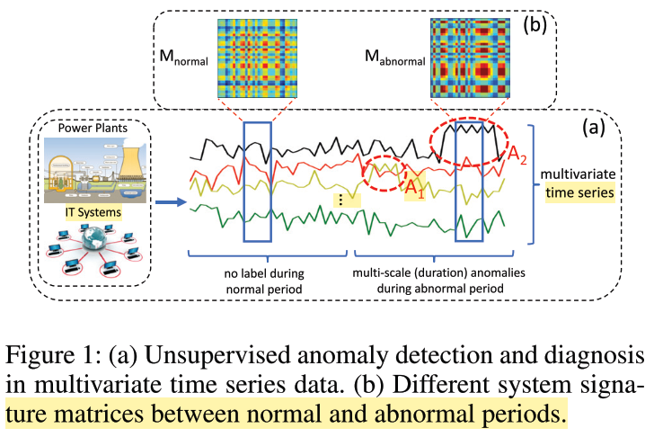
Figure 2 - Source: [2]

The graphical abstract for this picture is given in Figure 2. The basic idea of this model is similar to the VELC model in that it is also trying to reconstruct an input signal, and using the reconstruction error as an indication of whether or not that input is normal or anomalous. The MSCRED model also uses a variant of an LSTM to handle the time series data, similar to VELC. The difference is that the MSCRED model assumes that there may be useful correlations between different time series signals that we should look for in order to identify anomalies in the full dataset. Let’s take a closer view at the different components of the MSCRED model to understand how it looks for correlations across time series signals as well as within them [2].

The authors assume that the raw data is in the form of n time series that extend for T time; they also assume that the data is normal for time in the interval [0, T] but that the data input to the model after that time can be abnormal. Their real-world example is a power plant that has time series data from different sensors that together can be used to look for anomalies that could be indications of potential failures. But the input to the MSCRED is not the raw time series data. Instead, Zhang et al. compute the pairwise correlations between each time series and save that data in n x n signature matrices. It is these signature matrices that then become the input to the model [2].

The first component of the model is a convolutional encoder that is designed to look for correlations across the time series signals (i.e. for correlations between the entries in the signature matrix, where each entry is the correlation between two signals). This convolutional encoder learns to represent the spatial information in the signature matrices, and passes this on to an attention-based convolutional LSTM model (ConvLSTM). The authors explain that they adapted the original ConvLSTM model [3], which was able to learn the temporal information in a video sequence, but struggled to perform over longer time intervals. To mitigate this issue, they add an attention mechanism to the original ConvLSTM which allows it to selectively remember the relevant hidden states across time steps, increasing the memory of the model. Together, the attention mechanism and ConvLSTM are capable of finding both temporal and spatial patterns in the signature matrix, and they return feature maps indicating which elements in time and space are important to pay attention to. The feature maps are processed by a convolutional decoder and used to reconstruct the signature matrices. We use the residual of the signature matrices (i.e. the difference between the input and the output signature matrices) to compute a reconstruction score and identify which inputs are anomalies and which are normal. These scores help identify the anomalies, diagnose which signals contributed to the anomaly (i.e. root cause analysis) and the scores also contain information about the severity of the anomaly [2].

Paper 3: Learning to Simulate Complex Physics with Graph Networks by Sanchez-Gonzalez et al.

DeepMind delivers again with a beautiful paper on how graph networks can form the basis of a learned simulator that can model the physics of a variety of systems (i.e. from water to sand). This paper introduces a Graph Network-based Simulator (GNS) that uses a graph-based representation to model the physics of a system of particles. The authors argue that the value of building a learned simulator with artificial intelligence is that it can a) be built much faster, b) can run more efficiently (both in time and in memory allocation) and c) the simulator remains efficient when scaled up to larger systems [4].

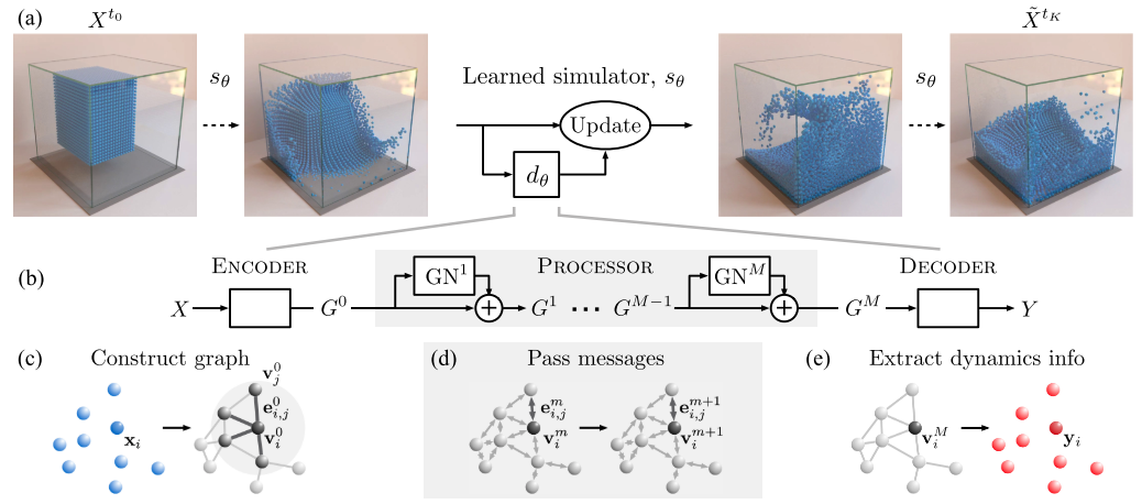
Figure 3 - Source: [4]

As shown in Figure 3, the overall architecture of DeepMind’s solution relies on a learned simulator that regularly updates the model of the system to accurately recreate the dynamics of a group of particles that represent water or sand or other fluid or rigid systems. In Figure 3, the simulator uses some learned dynamics, $d_{\theta}$, to update the states of all the particles and simulate their trajectories. The learned dynamics, \(d_{\theta}\), use a set of graph networks to learn the dynamics [4]. Let’s dive into the structure of \(d_{\theta}\) in more detail.

The dynamics are modeled using 3 key components: an encoder, a processor and a decoder. The encoder takes as input the first state of all of the particles in the system, and encodes that information into a graph in the latent space. This graph is then passed to the processor, which learns message-passing functions that connect all the nodes in the graph together (within a certain radius) and generates a series of output latent graphs that represent the progression of the system over time. The decoder extracts the relevant dynamics information (i.e. accelerations) from the final latent graph and passes them to an update mechanism, which in this case is a simple Euler integration function. In essence, this entire GNS is still using integration to solve the dynamics by stepping through sequential time steps - the only complexity comes in to how the dynamics are learned and represented and applied. The authors argue that this model is very general and so can be used to represent many different types of particle systems [4].

This all still felt a little general to me until I read deeper into the methods section to understand how each piece (the encoder, the processor and the decoder) were actually implemented. The encoder takes in the position, last C velocities and static properties of each particle and assigns one node to each particle. The encoder then learns functions to embed the input data into the nodes and edges of this graph. These encoder embedding functions are MLPs. The graphs embedded by the encoder are then passed to the processor which has a stack of M graphs with identical structure. The processor learns edge and node update functions, which are also MLPs. Finally, the decoder has a learned function (also an MLP) that is applied to each node on the final graph from the processor and outputs the second derivatives for each node to be passed to the update mechanism [4].

I also wanted to point out that I loved the way that this paper was written. Its figures do an excellent job of giving a high-level view of the architecture that is simple without losing too much resolution. The paper is written so that the reader spirals around the architecture, adding successively more detail on each pass. In total, I believe the authors went through the architecture three times, each time adding more information on the philosophy and implementation of the model design. This is something I would really like to do in my own writing.

References:

[1] Zhang, C., Li, S., Zhang, H., & Chen, Y. (2019). VELC: A New Variational AutoEncoder Based Model for Time Series Anomaly Detection. https://arxiv.org/abs/1907.01702v2

[2] Zhang, C., Song, D., Chen, Y., Feng, X., Lumezanu, C., Cheng, W., Ni, J., Zong, B., Chen, H., & Chawla, N. V. (2018). A Deep Neural Network for Unsupervised Anomaly Detection and Diagnosis in Multivariate Time Series Data. 33rd AAAI Conference on Artificial Intelligence, AAAI 2019, 31st Innovative Applications of Artificial Intelligence Conference, IAAI 2019 and the 9th AAAI Symposium on Educational Advances in Artificial Intelligence, EAAI 2019, 1409–1416. https://arxiv.org/abs/1811.08055v1

[3] Shi, X.; Chen, Z.; Wang, H.; Yeung, D.Y.; Wong, W.K.; and Woo, W.c. 2015. Convolutional lstm network: A machine learning approach for precipitation nowcasting. In NIPS, 802–810.

[4] Sanchez-Gonzalez, A., Godwin, J., Pfaff, T., Ying, R., Leskovec, J., & Battaglia, P. W. (2020). Learning to Simulate Complex Physics with Graph Networks.