We are back to our regularly scheduled programming! In other words, it is time to nerd out on a topic related to artificial intelligence again. Today I wanted to write a very quick post on binary cross-entropy (also called the log-loss function). I am currently learning to build a generative adversarial network (GAN) in TensorFlow. The tutorial computes the loss for both the generator and discriminator networks with binary cross-entropy. I wanted to better understand how this loss function works and why it is an appropriate choice for this application.

Setting Up The Problem

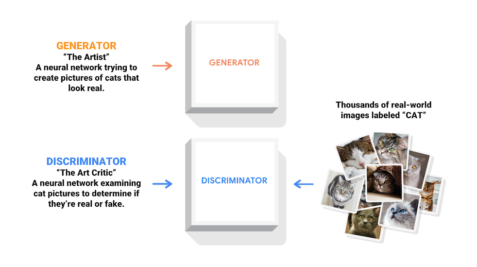
In this tutorial, I am working with the MNIST dataset of handwritten digits. I am training a generator neural network to create novel images that look like they belong in this dataset, and simultaneously, I am training a discriminator neural network to decide if an image that it sees belongs to the MNIST dataset, or is a novel image produced by the generator. This idea is demonstrated in Figure 1.

Figure 1 - Source [1]

As we have discussed previously, a neural network uses a loss function to update the weights of every node and improve its performance. In this case, the discriminator’s loss function is, conceptually, a sum over how well it was able to identify images that were from the real dataset, and how well it was able to identify “fake” images from the generator. The generator’s loss function is also a measure of how well the discriminator identified “fake” images - the generator is trying to trick the discriminator.

Using Binary Cross-Entropy as the Loss Function

Binary cross-entropy is used in binary classification problems, where a particular data point can have one of two possible labels (this can be extended out to multiclass classification problems, but that is not important in this context) [2]. It makes sense to use binary cross-entropy here because the discriminator can either label an image as “real” or “fake.”

We use binary cross-entropy as a measure of the loss of the neural network, or its error in making predictions. Large loss values (aka large binary cross-entropy values) correspond to bad predictions, and small loss values correspond to good predictions [2]. This measure of the loss is then used in backpropagation to update all the nodes in the neural network so that they perform better (i.e. make better predictions) on the next round. Let’s dive into how this works from a mathematical perspective.

The equation for binary cross-entropy is as follows [2]:

Equation 1

The labels for the data are y and p(y) is the probability distribution of the labels over the dataset of values, x [2]. But how did we get to this equation, and why does it intuitively make sense?

The Concept of Entropy

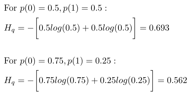
The idea of information entropy was introduced by Claude Shannon in the 1940s as a way of measuring the uncertainty, or surprise, contained in a data distribution [3, 4]. You can think of entropy as a measure of the predictability of a data distribution [4]. If it is equally likely that our discriminator will see “fake” or “real” images, then the distribution of images has maximum entropy [4]. But if we are more likely to see fake images than real ones, perhaps split (fake = 75%, real = 25%), then the entropy of the data distribution decreases because it is now more likely that we will see fake images [4]. Shannon gives a formula for entropy as follows [4]:

Equation 2

Notice that we use q(y) to represent the true distribution of the labels, y. We can see with our example above that the entropy of the equal distribution of real and fake images is larger than the entropy of the uneven distribution:

Equation 3

The Importance of Cross-Entropy

This is great, we can now mathematically describe the predictability of our data. But the problem with this approach is that it requires us to know the distribution of our data. And the entire point of training a neural network to discriminate between two datasets is because we do not know the distribution of our data. So we have to approximate the true distribution, q(y), with another distribution that we know and define explicitly, called p(y). Now I can rewrite my entropy expression using both my true distribution, q(y) and approximate distribution p(y) [2]:

Equation 4

Ideally, I want q(y) = p(y), because that would mean my approximation matches the real distribution precisely [2]. But I am never going to be able to approximate the true distribution perfectly, so I can expect that my cross entropy will always be greater than the entropy of the true distribution [2]. In other words, I know that [2]:

Equation 5

This expression is another way of writing the Kullback-Leibler Divergence, which we have seen before [2]. As a reminder, it can be written as [2]:

Equation 6

As p(y) approaches q(y), the KL divergence decreases, and our discriminator neural network gets better at classifying real and fake images. Given our understanding of the KL divergence in terms of Equation 5, we can see that if we minimize the cross-entropy, we will minimize the KL divergence and ultimately minimize our loss [2].

The neural network is doing exactly this by computing the cross-entropy as a sum over all the data points that it sees during training. Notice that to write the expression for the cross-entropy, we assume that the data is uniformly random, i.e. that [2]:

Equation 7

This allows the neural network to compute the cross-entropy loss as follows [2]:

Equation 8

After some manipulation, we can rewrite this function to be exactly the expression for the binary cross-entropy loss we presented in Equation 1 at the beginning of this discussion [2].

Conclusion

So in summation, the binary cross-entropy loss function is used in GANs to measure the difference between the distribution of predictions made by the discriminator, p(y), and the true distribution of the data that it is seeing, q(y). The binary cross-entropy measures the entropy, or amount of predictability, of p(y) given q(y). We try to minimize this cross-entropy because in doing so, we develop an improved approximation of the true distribution of the labels, q(y). I hope this explanation made sense, and please feel free to shoot me an e-mail with questions.

References:

[1] “Deep Convolutional Generative Adversarial Network.” TensorFlow. 12 Jun 2020. https://www.tensorflow.org/tutorials/generative/dcgan Visited 01 Jul 2020.

[2] Godoy, D. “Understanding binary cross-entropy / log loss: a visual explanation.” Towards Data Science on Medium. 21 Nov 2018. https://towardsdatascience.com/understanding-binary-cross-entropy-log-loss-a-visual-explanation-a3ac6025181a Visited 01 Jul 2020.

[3] “Entropy (information theory).” Wikipedia. https://en.wikipedia.org/wiki/Entropy_(information_theory) Visited 02 Jul 2020.

[4] Cruise, B. “Information entropy.” Khan Academy. https://www.khanacademy.org/computing/computer-science/informationtheory/moderninfotheory/v/information-entropy Visited 02 Jul 2020.