In the Machine Learning Coursera class by Andrew Ng, I am in the middle of understanding how to improve the learning performance of a neural network. Ng provides some fantastic guidelines on how to properly train a neural network and improve its performance, which I want to discuss here.

Divide Training Data into 3 Categories

When training a neural network, it helps to subdivide the training data available to train the network robustly. It is recommended that the dataset be divided into a training set (60% of the data), a cross-validation set (20% of the data) and a test set (final 20% of the data) [1]. By subdividing the data in this way we allow ourselves to find the best hypothesis that fits the data without overfitting. We will use each of the datasets to help us find the best order for the polynomial that represents our hypothesis by testing hypotheses with varying degrees [1]. As an example, let us say that we are testing three hypotheses that are second order, third order and fourth order polynomials, respectively. Here is how we would use each dataset [1]:

(1) Optimize the parameters, theta, for a neural network using each of the 3 hypotheses listed above with the training set.
(2) Check the performance of each of the neural networks with the “new” data in the cross-validation set and determine which neural network predicted the correct outputs with the lowest error. This step will show if any of the hypotheses are overfitting or underfitting, because the neural networks will be using data that they have not seen before and have not been able to fit themselves to.
(3) Calculate the error of the neural network that had the hypothesis with the lowest error in (2) using the test set.

Understanding Bias and Variance

When our model underfits or overfits to the data, that can be an indication if our model is exhibiting high bias (underfitting) or high variance (overfitting) [1]. Graphically, these concepts are shown in Figure 1 below. Let’s think about how the bias and variance of a model will change as we increase the degree of the hypothesis polynomial [1]:

(1) Training error: As the degree of the hypothesis increases, the training error should decrease because our model will get better at fitting to the data set.
(2) Cross-validation error: As the degree of the hypothesis increases, the cross-validation error will decrease to a certain extent, but then start to increase as the degree continues to increase. (Intuitively this might make sense if you think about the degree of the hypothesis polynomial as Goldilocks’ porridge. Make the degree too low, and the hypothesis will underfit, which will yield large errors; too high and the hypothesis will start to overfit and also have large error. The cross-validation error will only be low when the degree of the hypothesis is “just right.”)

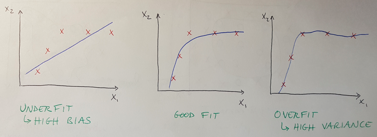Figure 1 - Inspired by [1]

These ideas are illustrated in Figure 2 below where we can see how the training error and cross-validation (CV) errors change with the degree of the hypothesis.

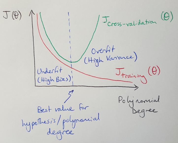Figure 2 - Inspired by [1]

Using Regularization to Avoid Overfitting

I recently introduced regularization, and I want to bring it back to this discussion because we can also use it here to deal with overfitting in our new workflow. Let’s say that we are going through the same workflow presented above, where we train multiple neural networks with hypotheses of degree 2, 3 and 4 using our three datasets: the training set, the cross-validation set and the test set. This time we are going to describe how we would modify this workflow so that we also find an ideal regularization parameter, lambda, that helps minimize bias and variance [1]:

(1) Choose a selection of values of lambda to test.
(2) Choose a series of degrees of hypothesis polynomials to test.
(3) Iterate through the values for lambda and for each value, train all the hypotheses of varying degrees on the training set.
(4) Calculate the cross-validation error for each neural network that has been trained with a given hypothesis degree and a given lambda. Be careful: while determining the cross-validation error, the model should NOT be regularizing the data (i.e. lambda = 0). We do this to control all variables while comparing cross-validation error across all of our neural networks.
(5) Choose the best combination of hypothesis polynomial degree and regularization parameter, lambda, that yielded the lowest cross-validation error.
(6) Apply the chosen hypothesis and lambda to the test set and check to see how well it performs.

Understanding the Network’s Learning Curves

Now let’s consider how we would use the different learning curves of a neural network to debug its performance. Keep in mind that, in general, when an algorithm is trained on a very small dataset (n =< 3) then the error will be 0 because we can generally always fit a quadratic or cubic curve to 3 points perfectly [1]. We will only see the training error increase as the network encounters 4, 5 or more data points. And in general, we will also tend to see the error plateau after encountering a large number of data points [1].

How would the learning curve look for a model that has high bias (i.e. is underfitting the data)? For the first couple of training data points, the training error will be low because the model will be able to fit to those few points [1]. As the number of data points increases, the training error will increase because it will not be able to fit to the data very well (it is underfitting) and adding more data points will not improve that situation [1]. Eventually the training error plateaus at a high value [1].

What happens when we calculate the error for a model with high bias during cross-validation (or testing)? (Note that the trends in error for both cross-validation and test phases are similar [1].) In this case, the cross-validation/test error will initially be very high because the model is encountering new data and needs to adjust its parameters accordingly [1]. However, since the model is still underfit, it will only be able to reduce its error by so much before the poor selection of hypothesis polynomial degree prevents it from making further improvements [1]. As the model sees more data points, the error will plateau at a high value [1]. All of this is shown in Figure 3.

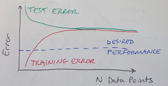Figure 3 - Inspired by [1]

In this situation, where our model is underfit to the data, we can see that acquiring more training data will not improve the situation, because our learning curves have simply plateaued [1]. Instead, we should consider choosing a larger hypothesis polynomial degree (i.e. increasing the number of features we include in our model) [1].

What happens in the other case, when the model is overfit and has high variance? In this situation, the training error will again start low and increase with more data points, and the cross-validation/test error will start high and decrease with more data points [1]. The difference this time is that the training error will continue to increase with more data points, and the cross-validation/test error will continue to decrease with more data points [1]. In this situation, acquiring more training data could help improve our model’s performance [1]. This is illustrated in Figure 4.

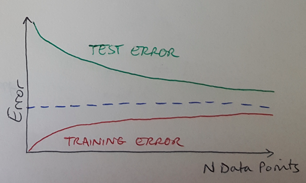Figure 4 - Inspired by [1]

[1] Ng, A. Machine Learning course, week 6 lecture notes. https://www.coursera.org/learn/machine-learning/home/week/6 Visited 02 May 2020.