Recently I have been looking into various topics on control and motion planning, and I wanted to just write a quick post to define some terms. I am also providing a somewhat detailed explanation of one control technique in particular, called model predictive control (MPC).

Definitions

First, some definitions. Visual servoing seems to be a somewhat generic term that describes any form of closed loop control that uses a camera to collect information about your system’s state [1]. There are two primary categories of visual servoing: (1) directly controlling the system’s degrees of freedom using information pulled from the camera feed and (2) geometrically interpreting the information from the camera feed before using it in a control loop [1]. This second method usually requires some knowledge about the shape of the system that is being observed with the camera so that we can draw conclusions about the system’s pose and orientation [1].

The second term that I hear all the time but have not got a great intuition for is trajectory optimization. Trajectory optimization refers to a broad class of methods that can be used to design a system’s trajectory which maximizes (or minimizes) some measure of performance, given some constraints [2]. Usually we perform trajectory optimization in an open-loop environment - that is, we assume that we will only be able to send commands to our system, but we will not necessarily be able to track the system’s state and respond to disturbances during the execution of the trajectory [2]. One simple example of this might be shooting a cannon ball (the control input is the angle of the cannon, which we want to optimize to hit our target).

We often use trajectory optimization when it is not necessary or practical to find a closed-loop solution to controlling our system [2]. We can also use trajectory optimization techniques when we only need to compute the first control step for an infinite-horizon problem (i.e. where we are trying to control the system forever) [2]. This last situation actually lends itself well to using model predictive control, which we will describe more below [2]. Some other methods of trajectory optimization include single shooting, multiple shooting, direct collocation, and differential dynamic programming [2]. I should probably write about all of these methods at some point, too.

Finally, I wanted to quickly explain linear-quadratic regulator (LQR) control. I have studied this technique multiple times and even implemented it myself on real hardware, but for some reason it always feels like a difficult concept to remember. LQR control is a way of finding a static gain, K, that can be used to perform feedback control according to u = -K x [3]. The matrix, K, is found by minimizing some cost function, J, which can be written as follows [3]:

Equation 1

Where U contains the control inputs at every time step, Q is the state cost, and R is the control cost [4]. In Equation 1, we are computing the cost over some horizon which is defined as N time steps [4]. The first term in the cost function computes the cost of the error between our desired and actual states at a given time step [4]. The second term computes the cost of applying a control input at a particular time [4]. Finally, the last term computes the cost of the error between our desired and actual final states [4]. The engineer must choose values for Q and R in order to optimize the controller for the particular problem at hand - this is often considered to be easier and more intuitive than other forms of controller design [5].

How do we use the cost function in Equation 1 to find our controller, K? If we assume that we can write the system dynamics as a linear system as follows [3]:

Equation 2

Then we can solve the associated Riccati equation for this system [3]. We use the solution, S, to write an expression for K [3].

Where did this Riccati equation come from? In general, we can define a Riccati equation as any first order ordinary differential equation that is quadratic in terms of the unknown function [6]. More specifically, for the particular case where we are designing a controller for our system’s steady state, we use the algebraic Riccati equation [6].

LQR is a very popular method of designing controllers and is often one of the first techniques you learn in a course on modern control theory. In the next section I’ll talk about MPC, which is another highly popular control algorithm, especially in recent years with the development of more powerful computers.

Model Predictive Control

Okay, now let’s dive into model predictive control (MPC) because it is a really cool tool that is getting a lot of air time in recent years in applications like drone control and autonomous vehicle control. MPC actually originated in the 1980s for use in chemical plants, because the processes occurring in the plants were slow enough that 1980s-era computers could perform the calculations needed to implement MPC [7].

Model predictive control does basically what the name advertises: it uses a model of the plant to make predictions about the future, and find the most optimal control input for the current time based on those predictions [7]. MPC assumes that you already know what your desired trajectory, or setpoint, is - in other words, we should already have done trajectory optimization for our application, and we are using MPC to make sure our system follows this desired trajectory. MPC is a computationally expensive approach - especially as the number of states gets larger and the control horizon is longer*1 - but as mentioned above, we can manage this to some extent with the more powerful computing resources we have today.

While PID control is still the dominant control strategy in industry, MPC is a better choice for MIMO (multi-input, multi-output) systems that have many inputs [7]. This is because PID controllers must be applied to each control input individually, and it can be challenging to tune the gains in each controller to optimize the entire system, because one control input could affect multiple output states [7]. MPC sidesteps this problem by optimizing the entire system at once [7].

Okay, let’s lay out the structure of the standard MPC algorithm, and then we will discuss how to choose some of the key parameters of the algorithm.

MPC Algorithm

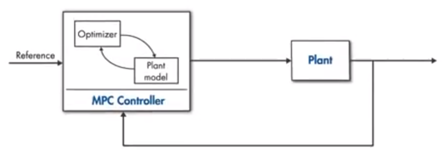
A brief block diagram of the MPC algorithm is shown in Figure 1. Here we are controlling some plant with our MPC controller, which contains two components: the plant model and the optimizer [8]. Our goal is to make the plant follow the reference, which could be a setpoint value or an optimized trajectory [8]. Let’s say we are designing an MPC controller for a car, and our goal is to make the car follow a trajectory which stays in the middle of a lane on the highway.

Figure 1 - Source: [8]

Our MPC controller works as follows: at the current time step, we use the model of the car to predict the car’s trajectory some number of time steps, p, into the future, assuming we give the car some control input, u [8]. In general, the controller will make this forward prediction for a number of possible control inputs [8]. The optimizer inside the MPC controller is using the predictions to find the sequence of control inputs that minimize some cost function [8]. The cost function is somewhat similar to Equation 1, and it is given below [9]:

Equation 3

The first term in Equation 3 computes the cost of deviating from the desired trajectory, and the second term is trying to minimize the control inputs so that we don’t abruptly apply large control inputs (this is generally a bad thing to do) [8]. The weights, w, are used to convey to the optimizer how important it is to minimize each cost [8]. For example, we may want to put more weight on minimizing the control inputs because our car is a passenger vehicle and we want our passengers to be comfortable. We can also apply constraints to the system’s control inputs and state: for example, we might say that you cannot turn the steering wheel more than 90 degrees, and the car cannot be allowed to move outside of its lane [8].

Once we have found the optimal sequence of control inputs, we apply the first control input in that sequence to the car [8]. Then we throw away all the rest of the control inputs, and move forward one time step [8]. On the next time step, we take a measurement of our system *2, and re-do the entire optimization process [8]. In this way, if there is some disturbance to our system that we did not predict, MPC is able to take that into account and generate a new sequence of control inputs [8]. Because we are constantly re-computing the control sequence at every new time step, MPC is also called receding horizon control [8].

Now that we have a basic idea of how MPC works, let’s talk about how we choose some of these parameters.

Parameter Selection

As we mentioned earlier, choosing the parameters for the MPC algorithm is important for ensuring that the computational complexity does not blow up and make solving the algorithm intractable [10]. But these parameters also affect the performance of the algorithm and how effectively it can control your application.

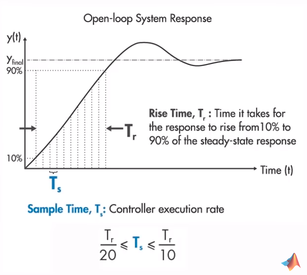
Let’s start by considering the sample time of the algorithm. If the sample time is too slow, then of course the controller will not be able to respond to disturbances quickly enough to avoid hitting one of the constraints [10]. For instance, you can imagine that if the controller for the autonomous vehicle is very slow, it will not be able to correct for a pedestrian in the road. Conversely, if the controller is too fast, then it might not be possible for it to finish a set of computations before the end of the time step [10]. MATLAB recommends choosing a time step that allows the controller to fit 10 to 20 steps into the open loop rise time of the system [10].

Figure 2 - Source: [10]

Let’s talk about the horizons of the algorithm. First we have the prediction horizon, which determines how many time steps into the future we need to compute a predicted trajectory using our model of the system [10]. If our prediction horizon is too short, then we fail to find a control policy that is truly optimal for our situation [10]. For example, imagine we are planning the autonomous vehicle’s speed as it approaches a bend in the road [10]. If our prediction horizon is not long enough to include the bend in the road, we may keep traveling at a high speed until the bend in the road is just ahead of us [10]. At that point, we will have to slam on the brakes which will be very uncomfortable for the passengers in the car [10].

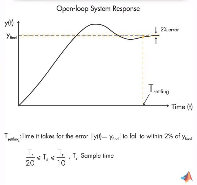
Figure 3 - Source: [10]

But so then why not just make the prediction horizon very long? Remember that we are still trying to avoid the Curse of Dimensionality - if we make the prediction horizon very long, then we are consuming a lot of computation resources and time to compute our next control signal [10]. Furthermore, remember that we’re going to throw away everything after the first time step and repeat this process, so it’s wasteful to have more computational steps than we truly need [10]. MATLAB recommends sizing the prediction horizon so that you can fit 20 to 30 time steps into the open loop transient system response [10].

The other horizon in the MPC algorithm is the control horizon [10]. This determines how many time steps into the future we need to compute our control sequence [10]. That is, when we are optimizing our control policy, the optimizer has to choose n control inputs, where n is the control horizon [10]. Again the Curse of Dimensionality comes into play here, because we can think of each control input as a separate variable that must be optimized [10]. Therefore, we don’t want to choose a horizon that is too long, because that will make the algorithm intractable. Similarly, if the control horizon is too short, we may not be looking far enough into the future to find the truly optimal control sequence [10]. In general, assuming that we are trying to reach some steady state setpoint, the first couple of control inputs are very important to our success, while control inputs that are in the more distant future will have less importance [10]. For the control horizon, MATLAB recommends choosing a control horizon that is 10 - 20% as long as the prediction horizon, and contains at least 2 to 3 time steps [10].

Finally, we can apply constraints to the MPC algorithm. We’ve touched on these already, but I just wanted to introduce the idea of hard and soft constraints [10]. Hard constraints cannot, under any circumstances, be broken by the algorithm [10]. On the other hand, soft constraints can be broken as needed, as long as the algorithm continues to try to minimize these states as much as possible [10]. Constraints can be applied to both the control inputs and the system’s states [10]. Let me illustrate the idea with another example. Let’s say that our autonomous car is fully loaded and has to climb a steep hill [10]. We apply a hard constraint to the control input - we cannot exceed some maximum input to the gas pedal - and we also apply a hard constraint to the car’s velocity - we cannot drop below the minimum allowable speed on the highway [10]. These hard constraints on both the control inputs and the state could produce an intractable situation where it is impossible to find a solution to the problem, because we cannot give the car enough gas to keep it moving at 45 mph [10].

The solution to this problem of hitting an intractable situation, is to never apply hard constraints to both the control inputs and the states [10]. If we had instead made the constraint on the car’s velocity soft, then we could find a solution to this problem, where the car would be allowed to slow down while it was climbing the hill, and then we would return to the desired speed after we returned to level ground [10].

Footnotes:

*1 The Curse of Dimensionality strikes again!

*2 Note that if we are lucky, we can directly measure the system state, but if that is difficult to do directly, we can also use state estimators like Kalman filters [8].

References:

[1] “Visual servoing.” Wikipedia. https://en.wikipedia.org/wiki/Visual_servoing Visited 26 Aug 2020.

[2] “Trajectory optimization.” Wikipedia. https://en.wikipedia.org/wiki/Trajectory_optimization Visited 28 Aug 2020.

[3] “lqr.” MathWorks. https://www.mathworks.com/help/control/ref/lqr.html Visited 28 Aug 2020.

[4] “Lecture 1: Linear quadratic regulator: Discrete-time finite horizon.” EE363 Stanford University. Winter 2008-09. https://stanford.edu/class/ee363/lectures/dlqr.pdf Visited 28 Aug 2020.

[5] “Linear-quadratic regulator.” Wikipedia. https://en.wikipedia.org/wiki/Linear%E2%80%93quadratic_regulator Visited 28 Aug 2020.

[6] “Riccati equation.” Wikipedia. https://en.wikipedia.org/wiki/Riccati_equation Visited 28 Aug 2020.

[7] “Understanding Model Predictive Control, Part 1: Why Use MPC?” MATLAB. YouTube. 15 May 2018. https://www.youtube.com/watch?v=8U0xiOkDcmw Visited 27 Aug 2020.

[8] “Understanding Model Predictive Control, Part 2: What is MPC?” MATLAB. YouTube. 30 May 2018. https://www.youtube.com/watch?v=cEWnixjNdzs Visited 28 Aug 2020.

[9] “Model predictive control.” Wikipedia. https://en.wikipedia.org/wiki/Model_predictive_control Visited 28 Aug 2020.

[10] “Understanding Model Predictive Control, Part 3: MPC Design Parameters.” MATLAB. YouTube. 19 Jun 2018. https://www.youtube.com/watch?v=dAPRamI6k7Q Visited 28 Aug 2020.