We have been talking a lot lately about implementing model predictive control (MPC) in discrete time. In this final post on the subject (for now), we are going to look at how we can write MPC as a convex optimization problem. We are going to use fast solvers in our codebase to solve MPC as an optimization problem, and so this post is intended to understand how to structure the MPC problem so it is easy to implement in code. We are going to start by discussing what convex optimization is (at a high level) and then work through the math of casting MPC as a convex optimization problem.

What is Convex Optimization?

Convex optimization is such a deep topic that there are entire graduate level courses on the subject, so I am going to make some generalizations here to avoid going into too much detail. Let’s start by considering what a convex function is: it is a function where you can draw a line segment between any two points and the line will always be above the curve, as shown in Figure 1 [1]. A convex function can only have one minimum, which is a key property that we exploit when we optimize these functions [1].

Figure 1 - Source: [2]

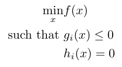
Convex optimization focuses on finding ways to minimize convex functions, and many of the solutions are polynomial time algorithms (this is good, algorithms of this order tend to be fast whereas in general finding function optima mathematically can be NP-hard) [3]. The standard form of a convex optimization problem looks like this [3]:

Equation 1

There may be zero, one or many solutions to this problem [3]. We can use tools like fmincon in MATLAB to perform convex optimization. In the next section, we will talk about how we formulate MPC as a convex optimization problem as given in Equation 1.

Writing MPC as Convex Optimization

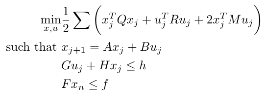
When we first encountered MPC, we learned that we needed to optimize some cost function, and that we had to constrain our optimization to account for the dynamics of our system. The problem was that our system dynamics were written in continuous time and it was impossible to write them in the form given for equality constraints shown in Equation 1. Now that we have learned about the discrete time formulation of system dynamics, however, it is possible for us to cast MPC as a convex optimization problem. Let’s start by writing out the basic form of the linear MPC problem in discrete time [4]:

Equation 2

The additional terms in the cost function (using matrices M and Q-tilde) add costs for the interaction between the state and the control input (in the case of the M matrix term) and for the terminal cost (in the case of the Q-tilde term). The additional constraints listed below the cost function allow us to define specific conditions we may need to consider for our particular system, such as the system dynamics. Please note that although we are describing the system dynamics in terms of A and B, these matrices are really phi and gamma, the discrete time equivalents of the continuous time matrices A and B.

We need a condensed form of Equation 2 to optimize, one that does not depend on the state at a particular time interval j [4]. Let’s see how we can aggregate the variables in the cost function and constraints into a different representation that only relies on the initial state [4].

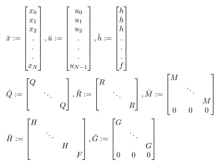
We start by writing the variables in the basic form (Equation 2) as vectors or matrices containing values for every time point we are considering [4]. Recall that in MPC we usually optimize over some horizon, so we will need as many entries as we have time points in our horizon. This looks like [4]:

Equation 3

This new representation will allow us to rewrite the minimization objective as [4]:

Equation 4

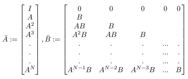
Notice that we can write the matrices A-bar and B-bar as follows [4]:

Equation 5

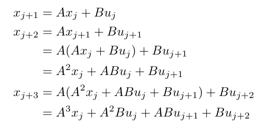
Why does this work? This works because, as we compute the values of successive states, we find that they only depend on the control inputs for each time point and the initial value of the state. Let’s see that in action over a few time steps:

Equation 6

Do you see how the pattern of the coefficients of the terms match what we have in Equation 5 for the A-bar and B-bar matrices? And do you see how, at every time step, we only need the initial state to compute our current state? This pattern now allows us to rewrite the dynamics as [4]:

Equation 7

Now we can substitute the system dynamics into the minimization objective and the constraints in order to get the following final expression [4]:

Equation 8

And there we have it, we have now successfully cast the MPC problem as a convex optimization problem in discrete time.

References:

[1] “Convex function.” Wikipedia. https://en.wikipedia.org/wiki/Convex_function Visited 8 Nov 2020.

[2] By Eli Osherovich - Own work, CC BY-SA 3.0, https://commons.wikimedia.org/w/index.php?curid=10764763 Visited 8 Nov 2020.

[3] “Convex optimization.” Wikipedia. https://en.wikipedia.org/wiki/Convex_optimization Visited 8 Nov 2020.

[4] Wright, S. J. “Efficient Convex Optimization for Linear MPC” in Handbook of Model Predictive Control, pp. 287-303. 2018. https://link.springer.com/chapter/10.1007/978-3-319-77489-3_13 Visited 8 Nov 2020.