Okay, it has taken us a little while to get to this point, but I think we are ready to introduce the Deep Deterministic Policy Gradient (DDPG) method of learning the policy function for a reinforcement learning situation. This approach was developed by a team from DeepMind and presented in 2016 by Lillicrap et al. [1]. In this post we will explain in some detail how DDPG works and then see how the MolGAN authors adapted it for their purposes.

DDPG (Finally)

Deep Deterministic Policy Gradient (DDPG) is a model-free, off-policy actor-critic method of solving policy gradient problems [1,2]. Let’s just break that down because that description tells us a lot. Model-free means we do not have a model for the dynamics, so we will have to learn the optimal policy without it. Off-policy means that we have a target policy that we are trying to learn, but we are actually exploring the action space using a second policy called the behavior policy. And actor-critic methods are methods where we are trying to learn the action-value function (critic) and the policy function (actor) simultaneously.

Remember: the goal in reinforcement learning is to find the optimal policy that maximizes the total return.

DDPG actually combines two approaches: DPG, as we saw last time, as well as the Deep Q-Network (DQN) method, which is capable of learning the Q-function via neural networks with great stability because it uses experience replay and other tools [1,2]. Both DPG and DQN methods give us tools that we need in order to solve the problem of learning the optimal policy for a continuous and large state space [1]. DPG gives us a means of finding the optimal policy in the continuous case, although the original method was designed for small state spaces [1]. Therefore we use DQN to give us the tools we need to apply neural networks in a robust manner to extend the DPG method to larger state spaces than it was originally designed for [1].

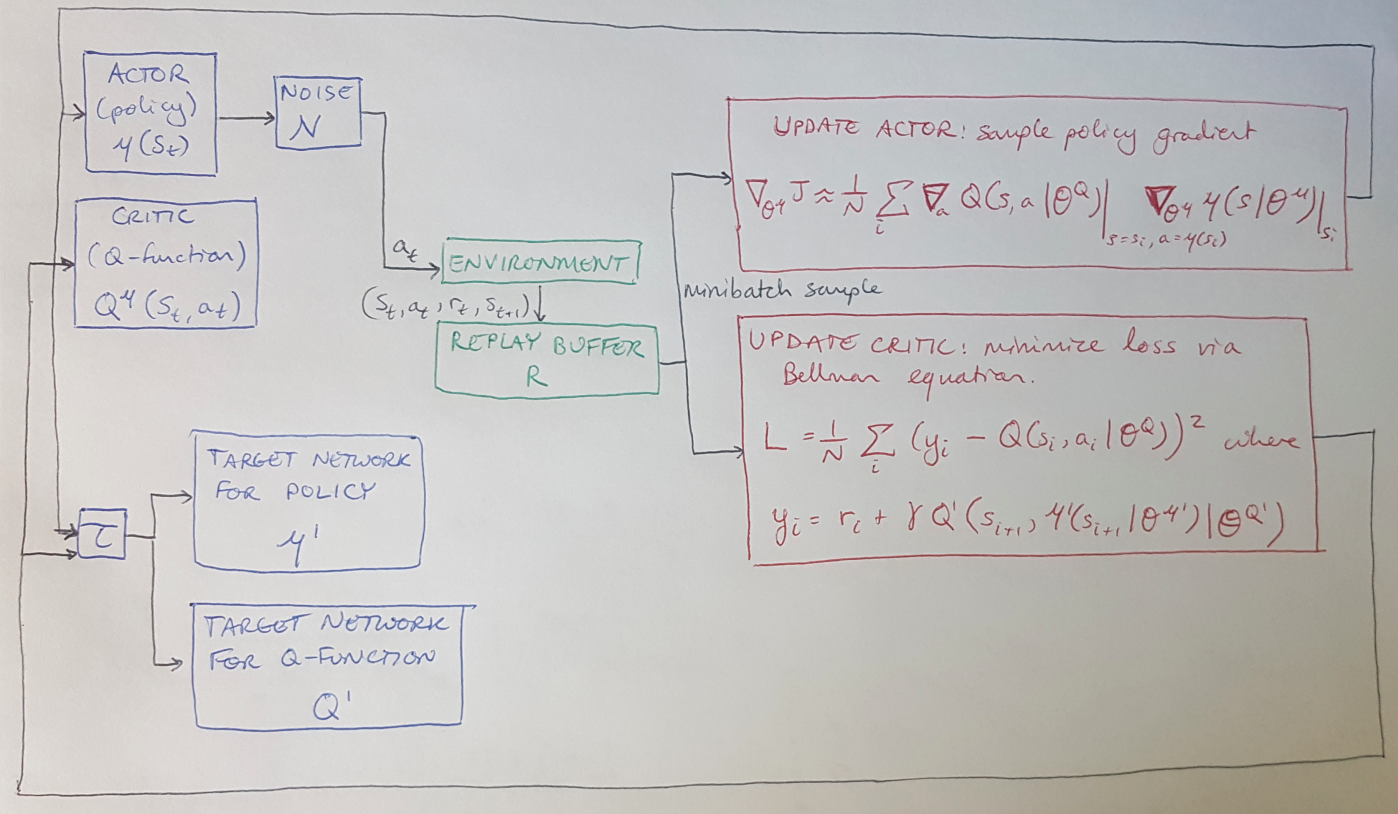
Before we dive too far into the explanation of DDPG, let me lay out the components of the algorithm, and then I will describe each one in detail and how they work together. We will have a total of four neural networks: the actor, the critic, and then corresponding target networks for the actor and critic [1]. We will interact with the environment and save tuples of the results in the replay buffer [1]. We will update the neural networks using the loss function and policy gradient shown in red [1].

Figure 1

First let me clarify that in the context of DDPG, the target policy that we want to learn and optimize is a deterministic policy, denoted by mu [1]. This is why we denote the Q value function in Figure 1 as being a function with respect to mu, not pi. I can write the equation for the Q value function as follows [1]:

Equation 1

In DDPG, the authors chose to define their deterministic target policy, mu as a greedy policy with respect to the Q value function [1]:

Equation 2

As we said previously, DDPG draws upon the DQN method, which is a form of Q-learning. Let’s briefly discuss Q-learning to understand how it is used here. Q-learning is an off-policy algorithm; the policy for this method is to maximize the Q-value (the action-value function) at every time step by following both a behavior policy (for exploration) and the target policy (for optimization) [1]. This is shown in Equation 3 below, and is covered in more detail in my other post. In DDPG, we will use a neural network to represent the Q function (i.e. the action-value function) [1]. We will train the Q function neural network by minimizing the loss as defined [1]:

Equation 3

Notice that we will call y the target function (this is not to be confused with the target policy) [1]. The target function, as we saw in the post on Q-learning, contains contributions from both the behavior and target policies, and helps to steer the optimization of target policy towards the optimal value while also allowing us to fully explore the state space.

Now we understand the architecture of the DDPG algorithm and we have seen how Q-learning has inspired the basic approach. The limitation of Q-learning is that we cannot apply it to continuous action spaces, because it would be computationally intractable to optimize the action at every time step [1]. Instead, we draw upon the actor-critic approach of DPG to help us optimize the policy and learn the Q value function [1].

The critic continues to be updated using the loss function (which follows the form of Bellman’s Equation), just as we showed above in Equation 3 [1]. The actor, however, now follows the gradient of the objective function that we showed in the previous post on DPG [1]. This method samples many trajectories and computes the expectation of the gradient over those samples [1]. Just for the sake of clarity, here again is the gradient of the objective function that we will use to update the actor [1]:

Equation 4

Okay, now we have laid out the theoretical underpinnings that allow us to optimize a policy for a large, continuous action space. Together, an intelligent combination of ideas from the DQN and DPG methods have given us new capabilities. However, there is one more set of problems that we must address with our new method. Since our goal in DDPG is to learn a policy for very large action spaces, we need a computational tool that will allow us to explore these large spaces. Using lookup tables to store the states and rewards will become computationally intractable - the Curse of Dimensionality dictates that the number of computations required per update using naive methods will exponentially explode [1]! So how can we explore large action spaces without explicitly keeping track of each and every action and state?

Lillicrap et al. propose that we use neural networks as function approximators for the Q value function and the deterministic policy, mu [1]. In their words, although “introducing non-linear function approximators means that convergence is no longer guaranteed […] such approximators appear essential in order to learn and generalize on large state spaces” [1]. The problem with using neural networks is that, historically, they can be unstable to train [1]. Lillicrap et al. use several tools, including a replay buffer, target networks and batch normalization to make the training process more robust and stable [1]. Let’s look into each of these tools in more detail to see how they help us to train neural networks per the DDPG algorithm.

The Replay Buffer

One problem with using neural networks in this context is that typical optimization algorithms for the weights assume that the training samples are independent and identically distributed (i.i.d.) [1]. Unfortunately, that assumption is not valid when the training samples are coming from sequential time steps over the same trajectory [1]. Also, in order to efficiently use our hardware, we will want to learn in minibatches, rather than from every sample in an online approach [1]. We can solve both problems using a replay buffer.

A replay buffer was introduced as part of the DQN method. It is a finite cache of tuples from the environment, where a tuple, as shown in Figure 1, is (s, a, r, s’) [1]. As the replay buffer is filled we discard the oldest values. During training, minibatch samples are pulled from the replay buffer and used to train the neural networks [1].

Target Networks

The second problem with training neural networks for DDPG is that the Q network can diverge [1]. This happens because, in the absence of a target network Q’, Equation 3 would use the value from the Q network in both the target, y, and the Q value itself [1]. The solution to this problem is to introduce a target network, Q’, which updates more slowly than the actual Q network [1]. These slow updates are also called “soft” updates, and they help improve the stability of the method’s learning process [1]. The authors point out that the presence of Q’ actually makes this problem more like a supervised learning problem, where Q’ is sort of like the true value that guides the learning process [1]. They also found empirically that the training process was more stable if they also introduced a target network for the deterministic policy, mu’ [1]. The soft update process can be expressed as follows [1]:

Equation 5

Batch Normalization

A third problem with applying DDPG to many different problems is that it can be hard to work with feature data that have very different ranges [1]. For example, it can be difficult to use the same hyperparameters for a DDPG algorithm that is used on a smaller, slower RC car as for a full size performance vehicle. The scales of the cars’ positions, velocities and accelerations would be different enough that the same hyperparameters would not work in both cases. Lillicrap et al. dealt with this problem by applying batch normalization to every dimension across the samples in a minibatch pulled from the replay buffer [1]. They also applied batch normalization to every subsequent layer in the neural networks [1]. They kept a running average of the mean and variance that were used to normalize the data, as well [1].

A Noise Process for Exploration

The final innovation of the DDPG algorithm is that the authors added noise to their deterministic policy in order to build their behavior policy [1]. The value of making the behavior policy stochastic is that it will explore new states that the agent may not otherwise see (recall our discussion of how Q-learning allows for exploration and exploitation) [1]. We can write this behavior policy as [1]:

Equation 6

It might be interesting to note that, while the noise could be any stochastic function, the authors chose to use noise generated by an Ornstein-Uhlenbeck process. Lillicrap et al. explain in the paper’s supplementary materials that an Ornstein-Uhlenbeck process is designed to model the velocity of a Brownian particle with friction, and this generates temporally-correlated values that have a mean of 0 [1]. I think that having temporally-correlated values that are unbiased was desirable for this algorithm.

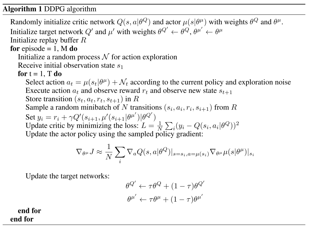
So now we should have some intuitive understanding of how DDPG works. We have seen how it combines ideas from DQN and DPG methods, and then makes use of several useful tools to make it possible to train neural networks to learn following this novel algorithm. The full DDPG algorithm is shown here [1]:

Algorithm 1

Tying DDPG Back to MolGAN

Now that we have done all this work to understand DDPG, let’s return to the MolGAN paper and understand how De Cao and Kipf implemented DDPG for their purposes.

If we recall from what feels like eons ago, the goal of the MolGAN algorithm is to generate novel graphs that represent chemical molecules and satisfy some desired properties, like solubility or druglikeness. The MolGAN architecture has a generator which produces novel graphs, and a discriminator that tries to guess if a sample graph is fake (i.e. made by the generator) or real (i.e. from the training data) [2]. De Cao and Kipf cast the generator as the policy of the MolGAN agent [2]. The policy chooses actions which in this case are graphs [2]. They clarify that there are no episodes in the MolGAN framework, because every episode is a single time step - that is, every episode consists of generating one novel graph [2].

So if the policy function is equivalent to the generator for MolGAN, what about the value function? De Cao and Kipf introduced a third neural network that learns a reward function by training against an externally generated real reward [2]. In other words, they had some external piece of software that could evaluate molecules for their properties, and they trained a neural network to approximate that code [2]. The advantage to representing the reward function with a neural network was that they could use the gradient of the neural network reward function to train the generator [2].

So now we have the actor-critic structure of DDPG, where the actor is the generator and the critic is the reward function. De Cao and Kipf also tell us that they chose not to use either experience replay or target networks in their implementation [2]. I think this makes sense because the DDPG architecture uses these tools to stabilize training over temporally-related, sequential, non-iid*1 data, but in the MolGAN case we actually do have iid data. That is, the graph-generation process is only one time-step long so there is no temporal dependency in the output data, and there is no real trajectory or episode, there is just one single action. So there is no need for experience replay or target networks. This means we essentially have a vanilla actor-critic architecture that uses neural networks as function approximators.

So if we don’t have experience replay or target networks, how do we modify the actor and critic updates as compared to the DDPG approach? The critic (the reward function) is trained using both fake and real data, and the true values used for supervised learning come from the external reward program that we discussed above [2]. So we would replace the target, y, in Equation 3 with the values from the external reward program. The reward function in MolGAN has essentially the same structure as the discriminator, the only difference is that it returns a score between 0 and 1 instead of some value between negative and positive infinity, as is the case for the discriminator [2].

The actor (the generator) is updated using a linear combination of the WGAN loss we discussed earlier and the RL loss [2]. The RL loss is the gradient of the reward function (aka the critic aka the Q value function) multiplied by the gradient of the generator (aka the actor aka the policy), per Equation 4 [2]. The MolGAN code base uses an interesting variation, which I do not fully understand, where they multiply the ratio of the generator loss to the RL loss against the RL loss [3]:

Equation 7

Note that in the code, the generator loss is equal to the least squared error between the real and fake feature weights from the discriminator [3]. I also do not understand why we are allowed to use feature weights for the generator loss, but we use the value of the logits returned from the reward function when given fake input as the RL loss [3]. I will need to figure this out in future!

But with that, I will finally conclude this series of posts, because we have hopefully now learned some intuition to explain how DDPG works and how it can be applied to the MolGAN problem.

Footnotes:

*1 Independent and identically distributed data = iid data.

References:

[1] Lillicrap, T., Hunt, J., Pritzel, A., Heess, N., Erez, T., Tassa, Y., Silver, D., and Wierstra, D. “Continuous Control with Deep Reinforcement Learning.” arXiv Prepr. arXiv 1509.02971, Sept 2015.

[2] N. De Cao and T. Kipf, “MolGAN: An implicit generative model for small molecular graphs,” arXiv Prepr. arXiv 1805.11973, May 2018.

[3] De Cao, N. “MolGAN.” Github repository. 21 Jun 2020. https://github.com/nicola-decao/MolGAN Visited 11 Aug 2020.