Our lab is working on implementing model predictive control (MPC) for an ongoing project, and so I have been learning the finer points of MPC in order to build this implementation. Since MPC is usually implemented with a computer, it is helpful to understand something about discrete time and how it affects our control algorithms. In this post, I am going to review some of the basics to help inform our understanding of MPC. I will start by explaining why we care about discrete time, the fundamentals of sampling in discrete time, and then introduce difference equations and (briefly) the z-transform. This is going to set up a discussion of how we can write a full dynamics model in discrete time in a follow-on post.

What is discrete time control and why do I need it for MPC?

Usually when we start learning about control theory, we think in terms of continuous time. Continuous time assumes that we can compute the value of a variable at an infinitesimally small period of time [1]. By contrast, discrete time assumes that we are sampling from a variable at regular instances in time, and that between each sample time, the value of a variable remains constant. Consider Figure 1, where continuous time is represented by the smoothly varying gray line, and discrete time is represented by the samples taken at the points indicated by the red arrows.

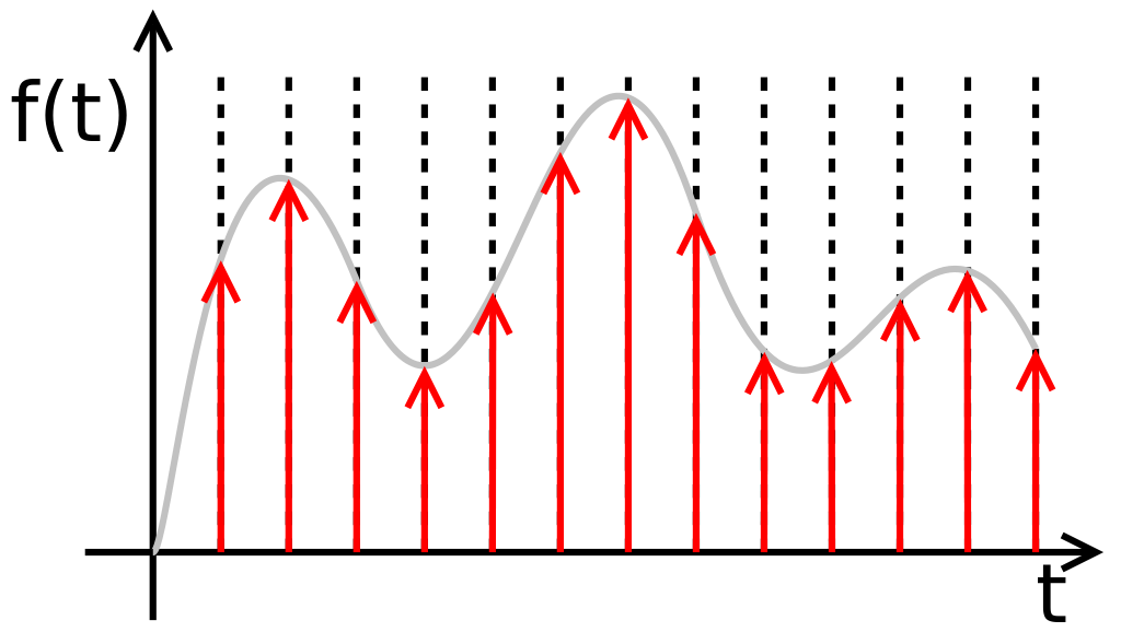
Figure 1 - Source: [2]

When we study control theory in continuous time, we use analytical expressions to describe our models that we can evaluate at any point in time. We can compute derivatives and integrals analytically, as well. We even learn to implement basic controllers like PID in continuous time, because it is possible to build PID controllers using only passive electronic components (resistors, capacitors, etc). Since these PID controllers are driven only by electric current (and not a computer chip), they will also operate in continuous time and the assumption of continuous time still holds.

But what happens when we need to implement MPC control? Can we continue to assume that we are operating in continuous time? No, we cannot, because MPC control requires a digital controller that can perform convex optimization. This means that we have to rewrite the mathematics behind MPC to accommodate for the fact that we are working in digital time, not continuous time. We have to take into account the fact that the computer is going to be sampling some signal from the plant at regular, discrete intervals, not continuously, and sending out control commands at regular intervals, too.

This difference is also shown in Figures 2 (continuous time control) and 3 (discrete time control). You can see that in continuous time, our error, output, control and reference signals are all in terms of continuous time, t, but in discrete time they are in terms of specific samples, k.

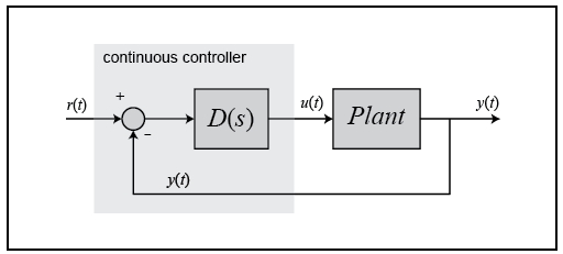
Figure 2 - Source: [3]

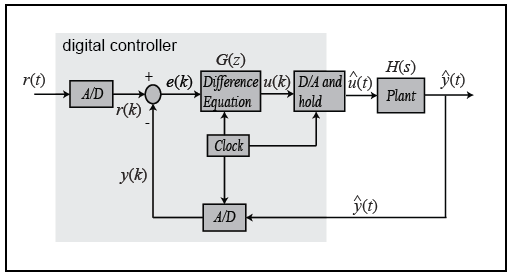
Figure 3 - Source: [3]

Basics of How Controllers Sample in Discrete Time

As you can see in Figure 3, we are using Analog-to-Digital (A/D) and Digital-to-Analog (D/A) converters to transition between discrete (digital) and continuous (analog) time [4]. Let’s think about how these converters might work in practice, starting with the A/D converter. This converter is operating on some physical signal, like a voltage taken from a temperature sensor. The A/D converter changes the voltage signal to some binary number that represents the voltage value. Depending on the resolution of the converter, the binary number will have a certain number of bits, often 10-12 bits. Let’s say the converter is a 10-bit converter. That means that it can encode 2^10 = 1024 discrete values. This is also like saying that we have a resolution of about 0.1%, because we can represent 1/1000th of a unit, which is also 0.1% [4].

The A/D converter, therefore, is converting the voltage signal to a binary number at regular intervals. More specifically, the converter has some sampling period, T, and we can say that the sample signal is in terms of these sampling periods, i.e. y(kT), where k is the integer number of samples we have taken so far. We can also shorten this to just write y(k), as shown in Figure 3, to indicate that we are working in discrete time now [4].

Similarly, the D/A converter is changing the discrete values output by the MPC controller into continuous time signals. Typically, this is done using something called a zero-order hold (more on this later), which just means that at regular intervals, we send a new command, u(kT), to the plant, and hold that value until the next sample time, when we send a different command. The zero-order hold just means that we hold the value of u(kT) constant over the sample period [4].

Now that we’ve briefly seen how we can change between discrete and continuous time, let’s discuss how a computer operates in discrete/digital time using difference equations.

Difference Equations

As we have seen before, our state space model for a dynamic system gives the model in terms of the derivative of the state variables, x. We need a way to write this derivative in terms of basic operations that a computer can perform, like addition, subtraction and multiplication, given a discrete set of samples. Once we have found a way to compute derivatives using only sampled, discrete points from a continuous-time plant, we will be one step closer to understanding how we must rewrite our continuous dynamics model into discrete time [4].

Recall that the definition of a derivative is [4]:

Equation 1

We can use Euler’s method to calculation an approximation of the derivative like so [4]:

Equation 2

Note that Equation 2 uses the forward difference method to compute the derivative, but we can also use the backward or central difference methods (central difference is generally recommended in practice, but the idea is the same in this discussion) [4].

Notice that Equation 2 is written solely in terms of values that the digital controller has access to: specifically, sampled points in time and the sampling period, T. This means that any time we encounter a derivative within the MPC implementation, we can now use Equation 2 to compute it. And if our system’s bandwidth is small, and our sampling period is sufficiently fast, we can assume that our approximation errors will be very small [4]. Let’s see how Equation 2 could be used to rewrite the dynamics model in discrete time [4]:

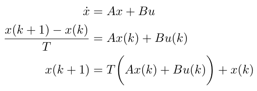
Equation 3

In general, sampling introduces a small delay in our system of value T/2. The delay can be approximated by a first-order Pade approximation as [4]:

Equation 4

Note that the sampling delay reduces the system phase. More intuitively, we can say that delays reduce system damping and system stability. In the next section, we will talk about how we can start to introduce the sampling delay into our dynamics models using the z-transform [4].

The Z-Transform

In this last section, we are going to introduce the z-transform. So far we have seen that in continuous time, we consider signals as a function of continuous time, t, such as y(t). Similarly, we have seen that we can consider discrete time-based signals as functions of k, such as y(k). We know that in continuous time, we can convert from the time domain (t) to the frequency domain (s) using the Laplace transform. Sometimes we want to analyze a system in the frequency domain because it can be a more intuitive way to think about system stability and controller design. Similarly, the z-transform is a way of converting from k to z, where z is, conceptually, equivalent to s [4].

Recall that the Laplace transform can be written as [5]:

Equation 5

Similarly, we can write the z-transform as [4]:

Equation 6

In this case, e represents the error signal into a system, and the bounds on z describe the values of z for which the sum converges [4].

Using this z-transform, we can now convert from the discrete time domain, to the frequency domain in terms of z. This allows us to write transfer functions in terms of z, taking into account the phase shifts caused by sampling delays in discrete time [4].

Now that we have gotten a brief introduction to some of the key concepts in discrete (or digital) time, we will next explore how we can rewrite a dynamics model from continuous time to discrete time. We will then take this model and look at how we can use it in writing the convex optimization formulation for MPC control.

References:

[1] “Discrete time and continuous time.” Wikipedia. https://en.wikipedia.org/wiki/Discrete_time_and_continuous_time Visited 01 Nov 2020.

[2] By No machine-readable author provided. Rbj assumed (based on copyright claims). - No machine-readable source provided. Own work assumed (based on copyright claims)., Public Domain, https://commons.wikimedia.org/w/index.php?curid=870308

[3] “Introduction: Digital Controller Design.” Control Tutorials for MATLAB & Simulink. https://ctms.engin.umich.edu/CTMS/index.php?example=Introduction&section=ControlDigital Visited 01 Nov 2020.

[4] Franklin, G., Powell, J., Workman, M. “Digital Control of Dynamic Systems, 3rd Ed.” Ellis-Kagle Press, Half Moon Bay, CA, 1998.

[5] “Laplace transform.” Wikipedia. https://en.wikipedia.org/wiki/Laplace_transform Visited 01 Nov 2020.