In the last post, we introduced a new paper presenting an object-centric perception, prediction and planning (OP3) learner [1]. We ended the post by noting that this learner must approximate a posterior predictive distribution of observations using Bayesian variational inference [1]. In this post I am briefly going to summarize Bayesian variational inference and then explain how it is used in this paper. If you want to see another machine learning tool that uses variational inference, please take a look at my posts about variational autoencoders.

Bayesian Variational Inference

We use Bayesian variational inference when we want to approximate a posterior distribution that would otherwise be difficult to compute [2]. Let’s describe the posterior distribution in terms of a filtering problem, where we are trying to predict our state (which we cannot directly measure) using a model and some measurement data. The posterior distribution, in this case, is a probability distribution that gives our prediction of our current state given our dynamics model, the likelihood of our data, and some evidence. The posterior distribution is described using Bayes’ Theorem as shown in Equation 1 and Figure 1 [3]:

Equation 1

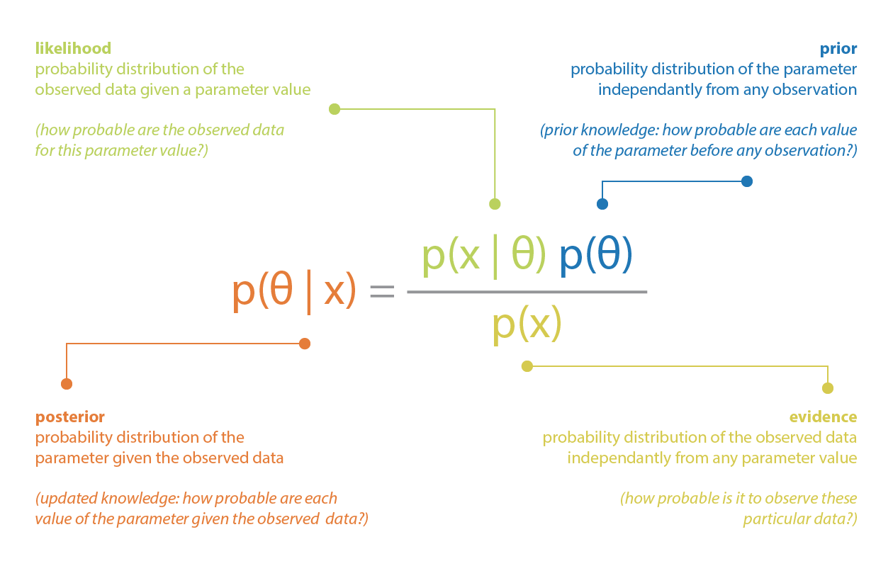
Figure 1 - Source [3]

The thing that makes the posterior distribution difficult to compute directly is the denominator - we call this the evidence, or the normalization factor [3]. In order to compute the evidence, we need to integrate the following expression over all possible values of X (where X represents the underlying state that we cannot directly measure but we can represent with a dynamics model) [3]:

Equation 2

This integration might be easy at low dimensions (for example, if you are working with toy problems like coin flips or dice rolls) but it quickly becomes intractable at higher dimensions [3]. So as an alternative we can use variational inference, and for the purposes of this discussion, let’s assume that we are working with normal (or Gaussian) distributions, although this method can be used with any distribution.

Let’s say we want to approximate a posterior P(X given Z), and we are going to use a family of Gaussians, Q(q), which can be parameterized by lambda. The i-th value of lambda just contains the mean and standard deviation which can be used to fully describe the i-th Gaussian curve q selected from the family Q. In mathematical terms:

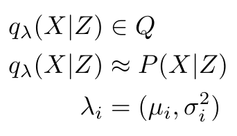
Equation 3

I want to minimize the difference between my approximate Gaussian curve, q, and the actual posterior, P(X given Z). I can calculate the difference between two distributions using the Kullback-Leibler divergence (KL divergence) which is defined as follows:

Equation 4

A small value for the KL divergence indicates a small difference between the two distributions. So if I want my approximation to represent my posterior as closely as possible, I need to minimize the KL divergence, as follows:

Equation 5

But the struggle continues, because this expression still includes finding P(X), which we already said was intractable. So let’s define a new term, the Evidence Lower Bound (ELBO), which is just the first 2 terms in the expression for the KL divergence in Equation 4:

Equation 6

Now let’s substitute the ELBO back into the expression for the KL divergence:

Equation 7

Now we can see that if I want to minimize the KL divergence, I only need to minimize the ELBO term, which is a function of my approximation q’s parameters, lambda. I don’t need to minimize P(X) because it is just some constant term. This is how we can use the ELBO to approximate a posterior distribution without having to perform any intractable computation.

One more note: I can also write the ELBO in this way (this will be useful in the next section) [4]:

Equation 8

How OP3 Uses Variational Inference

The OP3 learner uses variational inference to approximate three distributions: (1) an observation distribution, G, (2) a dynamics distribution, D, and (3) a recognition distribution, Q* [1]. We can define each of these distributions as follows [1]:

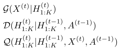
Equation 9

The authors define the ELBO for their learner as follows [1]:

Equation 10

Veerapaneni et al. explain that by maximizing this formulation of the ELBO, they can encourage the recognition distribution, Q, to return entity states that will be useful to the observation distribution, G, as well as to the dynamics distribution, D, which is trying to predict future states of the entities [1].

OP3 will use these three distributions (the observation, dynamics and recognition models) to approximate the posterior predictive distribution, by maximizing the ELBO defined in Equation 10 [1]. Notice that last time, we saw that we could generate a series of observations and entity states from a sequence of actions (which we would use in the posterior predictive distribution, as well) by writing the following expression [1]:

Equation 11 - Source: Equation 1 in [1]

As we discussed before, this expression explicitly uses the observation and dynamics models, which we are trying to optimize with the ELBO [1]. (The recognition distribution, Q, is implicitly used in the OP3 learner to help improve both the observation and dynamics models [1].) Let’s look at each model in turn and understand where they come from.

Observation Model, G

The observation model is approximating P(X given H), which is a term in Equation 11, as we discussed above. The observation model can be written as follows [1]:

Equation 12 - Source: Equation 2 from [1]

Here, we can see the entity abstraction coming into play, because the entire observation model is a sum over all of the individual entities that the learner has identified in the scene [1]. The function g(X given H) is called an entity-centric function, and it models how each entity is generated [1]. We assume that each entity, H, can be represented as a mixture of models at every pixel in the image, where the pixel indices are (i,j) [1]. The weights for each model are represented by the function m, and are computed based on the relative distance of each entity from the camera [1]. A diagram of the observation model is shown in Figure 2.

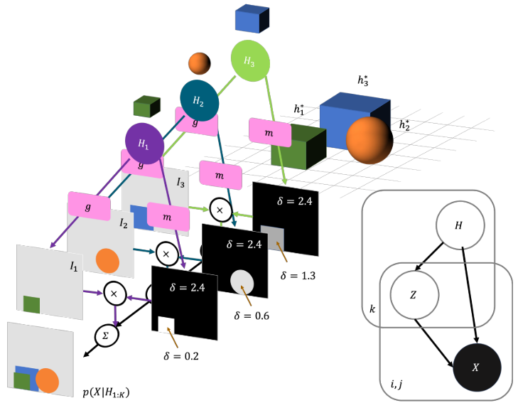
Figure 2 - Source: Figure 3 from [1]

Dynamics Model, D

The dynamics model is approximating P(H’ given H, A) where H’ is the set of future values for the entities’ states [1]. This is the other term that appears in Equation 11 as shown above. The dynamics model is a bit more involved than the observation model, but it still follows the entity abstraction methodology by considering each entity individually [1]. The dynamics model needs to consider several sets of interactions for each entity: (1) the individual dynamics of an object, d-o, (2) the effect of the action on the object, d-ao, (3) the pairwise interactions between objects, d-oo and (4) the aggregation of all of these interactions, d-comb [1]. (The dynamics model also uses a function to embed the action vector into this model, d-a [1].) We can see an illustration of how these interactions are considered in Figure 3. Notice that each of these interactions is represented as a generic function - we use generic in this context to mean that we apply the same function to all entities [1]. The reasoning for using a generic function is that if these dynamics functions represent physical laws, the same physical laws would apply to all objects in the environment, just as gravity applies to all objects on Earth [1].

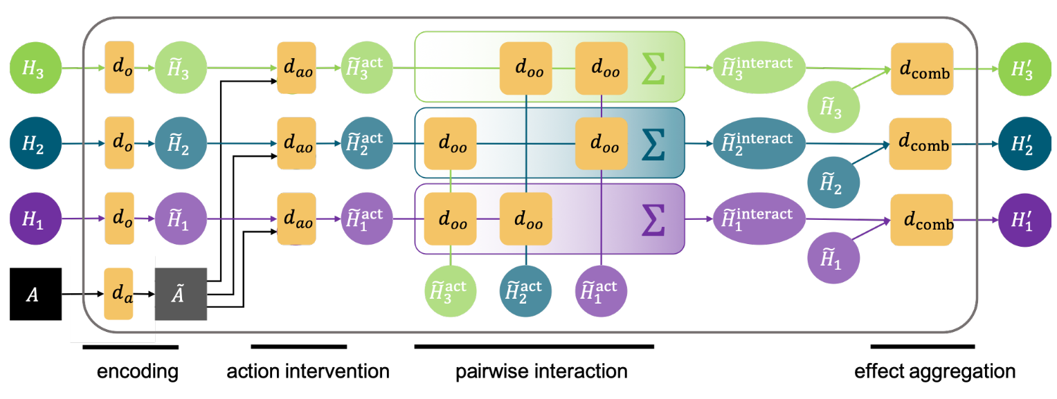
Figure 3 - Source: Figure 4 from [1]

We can write a general, abridged form of the dynamics model as follows [1]:

Equation 13 - Source: Equation 3 from [1]

The cool thing about this approach is that it scales very well to numbers of objects that the learner may never have seen in training [1]. The same set of functions can be reused across an infinite number of entities [1]. The one thing that I am not sure about is how computationally expensive this approach could get if we were trying to learn from an environment that contained a large number of objects that interacted - wouldn’t that generate a large combination of computations that we would have to calculate? Wouldn’t that still be expensive even if the function we used to calculate the interactions was the same for all entities?

At any rate, we almost have the full picture of how OP3 works now. The final piece of the puzzle is understanding exactly how the learner matches objects in the video frames to entities in the latent space. It does this using something called “amortized interactive inference,” which we will discuss in our next and final post [1].

Footnotes:

*The recognition distribution helps to update the states of the entities, along with the dynamics model. We will look at it in more detail in the next post.

References:

[1] R. Veerapaneni et al., “Entity Abstraction in Visual Model-Based Reinforcement Learning,” Oct. 2019. ArXiv ID: 1910.12827 https://arxiv.org/abs/1910.12827

[2] D. M. Blei, A. Kucukelbir, and J. D. McAuliffe, “Variational Inference: A Review for Statisticians,” J. Am. Stat. Assoc., vol. 112, no. 518, pp. 859–877, Jan. 2016.

[3] Rocca, J. “Bayesian inference problem, MCMC and variational inference.” 01 Jul 2019. Towards Data Science, hosted by Medium. https://towardsdatascience.com/bayesian-inference-problem-mcmc-and-variational-inference-25a8aa9bce29 Visited 20 May 2020.

[4] Wikipedia. “Evidence lower bound.” https://en.wikipedia.org/wiki/Evidence_lower_bound Visited 20 May 2020.