In today’s post, I want to discuss the basics of linear regression and gradient descent. These are two basic tools used in supervised learning (as discussed in my previous post). Linear regression is used to fit a mathematical function (like a line or a parabola) to a set of data [1]. And gradient descent is used to find the local optima of such a function [1].

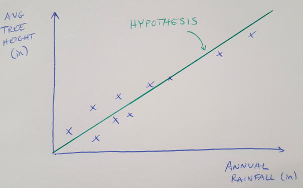
Figure 1

Let’s begin with linear regression, and a basic example. Let’s say we are trying to find a function that maps the relationship between annual rainfall and tree height in a forest. We plot the data on an x-y plot as shown in Figure 1. We are going to start by trying to find a linear relationship, because the points seem to fall along a straight line. It is also better to start by finding a simple relationship and adding complexity later. We call this function or relationship our hypothesis, and we can write an expression for the hypothesis as follows [1]:

Equation 1

We call the variables theta1 and theta2 the parameters of our hypothesis [1]. We can change the values of our parameters to make the hypothesis fit the data as closely as possible. And we can quantify how well our hypothesis fits our data with a cost function, J, as written below [1].

Equation 2

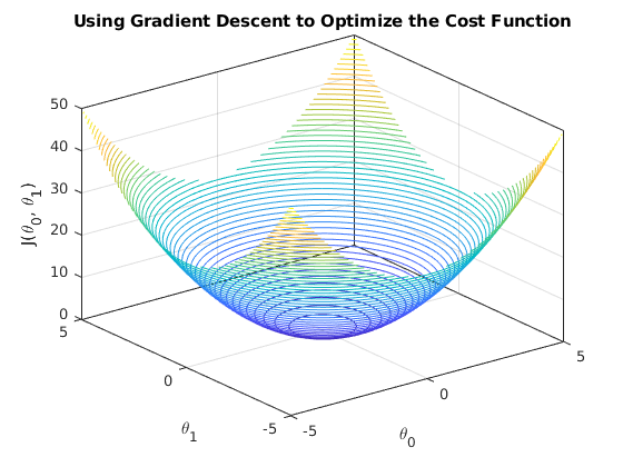
The purpose of linear regression is to find a set of parameters that minimize the cost function J [1]. But how do we do that? This is where gradient descent comes into play. Let’s plot the cost function J as a three-dimensional surface that maps out the value of J for all values of the parameters theta0 and theta1, shown in Figure 2 [2]. Do you see how this surface is shaped like a bowl, with a low point in the middle? That is the global minimum of the cost function, and it represents the point where our hypothesis will fit the data the best [1]. We will use gradient descent to find the values of theta0 and theta1 that correspond to this global minimum [1]. Note that linear regression always has a convex cost function (i.e. it has only one global minimum, no other local minima) so we say the cost function J is a convex quadratic function [1].

Figure 2 (Source code from [2])

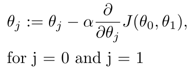
The process of gradient descent is simple - we are going to change theta0 and theta1 repeatedly until we find the minimum of J [1]. But we are going to do this intelligently - we will update our theta0 and theta1 parameters so that they are always reducing the value of J. We can do this by following the gradient of J [1]. Recall that the gradient tells you the rate of change of J in a given direction. So if we know the gradient of J in the direction of theta0 and theta1, we can follow it “downhill” until we come to the global minimum. Here’s how we will do that in mathematical terms [1]:

Equation 3

The alpha term shown in the equation above is the learning rate, which we encountered a couple of days ago in my introduction to reinforcement learning post. In this situation, alpha determines how big of a step we take down the hill [1]. Tuning alpha is important in gradient descent: if the value of alpha is too small, gradient descent can take a long time because you are taking really small steps towards the global minimum [1]. If alpha is too large, you can miss the local minimum and end up not converging, or diverging (imagine zig-zagging up the bowl instead of down towards the middle) [1]. With alpha fixed, gradient descent algorithm still takes smaller steps as it approaches the local minimum because the derivative term gets smaller as the slope gets shallower, and you get this for free without having to adjust alpha [1].

References:

[1] Ng, Andrew. Machine Learning course, week 1 lecture notes. https://d18ky98rnyall9.cloudfront.net/_ec21cea314b2ac7d9e627706501b5baa_Lecture2.pdf?Expires=1576195200&Signature=ju60TNphbauBhv3R3OwowzYtxs8wHZbt-d27TW~R-ufWqlJuoLeTRAS76jzaoYIJsHSV-vOIvvTtm8u~IZd2TvwyC95GySvthxjA4AGVsvOEjSBkSY7aLrVIE8BC-mgFBLdMjWPpwxm~6UXy5cKp3LBP7n5~QbdUzQXhh68ygi4_&Key-Pair-Id=APKAJLTNE6QMUY6HBC5A Visited 12/11/2019.

[2] MATLAB. “contour3.” MathWorks Documentation. https://www.mathworks.com/help/matlab/ref/contour3.html Visited 12/12/2019.