I am still finding linearization a tricky subject, but I had to linearize an inverted pendulum system for a class this weekend, and going through that process helped me to clarify for myself how linearization should work [1],[2]. If you haven’t read it already, please start with my earlier post on the fundamental concepts behind linearization.

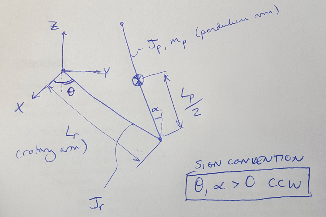
In this post, we are going to linearize the equations of motion for a pendulum about the inverted position (i.e. where the pendulum is pointing straight up). We have two degrees of freedom in this system: theta describes the angle of the rotary arm that spins in the x-y plane, and alpha describes the angle of the pendulum which rotates in the y-z plane (see Figure 1 below for a schematic). We have a single control input, the torque, tau, which is input to the system at the base of the rotary arm. You could say that this system is underactuated because we have more degrees of freedom than we have control inputs.

Figure 1

My ultimate goal is to obtain the state space equations for this system so that I can design a controller for it. The state space equations for a plant are [1],[2]:

The first equation encapsulates my system dynamics, and matrices A and B describe how my plant responds to changes in state and changes in control input. The second equation describes my system outputs as a function of the states and the control inputs. We are going to focus on the first equation for this discussion about linearization (the second equation is determined by my setup and which state variables I am able to measure; that’s a conversation for another day). I can write two equations of motion for this system, describing the acceleration of the two angles, theta and alpha:

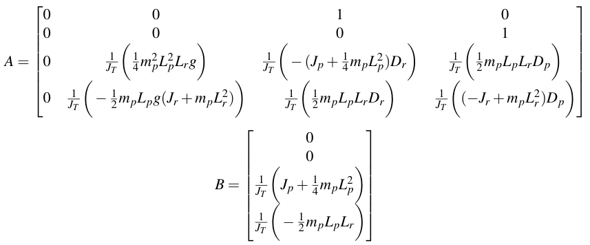
Once I have these equations (in this case the manufacturer used the Lagrange method to obtain them, and I have written an earlier post on obtaining equations of motion), I can linearize them. But notice that each equation depends on multiple state variables. (The state variables include theta, alpha and their velocities, theta-dot and alpha-dot.) So I need to linearize each equation with respect to each state variable, and then compile all the linearized equations into the matrices A and B.

This is where I was confused before I wrote this post. In solving our practice exams, we often found that we only needed one linearized equation relating one state variable to the control input. I was confused by that - how exactly was I supposed to know which equation I should linearize for which variables? Now I know that I should look for the equation that contains both my state variable of interest and the control input. I suppose now I am just not sure what to do when I have two such equations that meet these requirements? I will post the answer in the future once I’ve figured it out. In the meantime, you can see my resulting A and B matrices below.

References:

[1] Quanser. “Modeling Documentation: QUBE-SERVO 2 Inverted Pendulum.”
[2] Quanser. “QUBE-SERVO 2 Workbook - Student.”