As part of a project I am working on, I have encountered the two concepts of the maximum likelihood estimate and the maximum a posteriori estimate. I don’t really understand their significance (although we have touched on the maximum likelihood estimate, or MLE, in our discussions of VAEs and filtering), so I wanted to write a post dedicated to describing these two ideas and their tradeoffs. The first thing to understand about both of these ideas is that they are both ways to estimate the parameters for a model of a process [6]. These concepts are based in probability theory and Bayesian inference, but I am interested in them because they are also powerful ideas in machine learning and related topics. In this post, I will start by describing MLE because we have seen it before, and then introduce the maximum a posteriori estimate (MAP) as a generalization of the MLE approach. But first, we’ll start with some basic terms.

Fundamentals

As we mentioned in a previous post, a statistical model is meant to describe a process using data. All models have some parameters that fit them to a particular dataset [1]. A basic example is using linear regression to fit the model y = m*x + b to a set of data [1]. The parameters for this model are m and b [1]. We are going to see how MLE and MAP are both used to find the parameters for a probability distribution that best fits the information we have available.

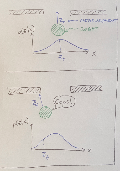
One more term needs clarification before we move on: likelihood. In our wall-following robot example we saw that the likelihood of getting a measurement, z, is the probability that we would have gotten that measurement if we were at a certain location, x, along the wall. This idea is illustrated in Figure 1. The likelihood function will tell us the chance we have of getting a particular measurement, z, at every possible location, x. In other words, we are trying to find a model for the process that was most likely to have given us that data.

Figure 1

Likelihood is different from probability [2]. Probability describes the chance that we will get a certain result, whereas the likelihood tells us how likely a certain hypothesis is to be correct [2]. For example, the results of a coin toss are described by a set of probabilities [2]. These probabilities are “mutually exclusive and exhaustive” - that is, the probability of getting a heads excludes the chance of getting a tails, and the total probability of both of those outcomes sums to 1 [2]. On the other hand, hypotheses are neither mutually exclusive, and it can be very hard to come up with an exhaustive list [2]. For example, if I guessed the sequence of 10 coin flips correctly 70% of the time (that is, if I got 7 out of 10 guesses correct), there are a lot of hypotheses to explain why that happened [2]. Maybe it was a fluke, I just got lucky; maybe I am able to predict the future a little bit; or maybe I had a bad radio connection to Martians who were able to predict the outcomes and communicate them to me [2]. We can compute the likelihood for each of these hypotheses, but the likelihoods do not add up to 1, and there are more possible hypotheses which I did not list, and which could possibly incorporate the hypotheses I made here [2]. If I want to learn anything meaningful from the likelihoods for different hypotheses, I need to compare the likelihoods for two or more hypotheses using the Bayes factor [2]. For example, the hypothesis that I got lucky might be 10 times more likely than the hypothesis that I can see into the future. This is another perspective on the difference between likelihood and probability.

Maximum Likelihood Estimate

Now that we have nailed down some of these basic concepts, let’s introduce the maximum likelihood estimate. This method is trying to maximize the likelihood that the process I am modeling would have given us some measurements [1]. As an example, let’s say my wall-following robot collected three measurements of its distance to the wall using a sensor [1] - I measured 5 m, 10 m and 11 m. I want to maximize the likelihood that I got these three measurements [1]. In other words, I want to find P(Z = 5, Z = 10, Z = 11 given X) and maximize it [1]. I am going to make some assumptions so that this is easier to do: first, I will assume that my likelihood can be modeled as a Gaussian distribution [1]. Secondly, I will assume that the three measurements I took are independent of each other, which allows me to simplify the likelihood as follows [1]:

Equation 1

I can do this because the measurements are independent - that is, they are not conditional on one another, so I simply multiply the likelihoods of each individual measurement together. A quick note: it might seem confusing that the likelihood is represented by some distribution P( ) - this follows the convention set by Bayes’ Theorem that we write the likelihood as P(Z given X) where Z is some measurement given that we are at some position X.

Since I know that the likelihood of each measurement can be written as a Gaussian distribution, I can rewrite Equation 1 as follows:

Equation 2

Now that we have an expression for the likelihood, we can find its maximum by taking the derivative and setting it equal to 0 [1]. But this is a little challenging to do with Equation 2, so to make the math easier, I can take the natural log of this expression (we call this the log-likelihood) and then take the derivative [1]. Why is this valid? This works because the natural log is a monotonically increasing function; when we find the maximum of the log-likelihood, it will occur at the same values of mu and sigma that we would find if we took the derivative of the likelihood [1]. The only difference is that the math is easier here. Let’s see that in practice [1]:

Equation 3

Then I take the partial derivative of this expression with respect to mu, and I set the partial derivative to 0 to find the value of mu that maximizes the likelihood [1]:

Equation 4

I would use the same approach to find sigma, and then I will have a complete description of the maximized Gaussian distribution that represents the model that is most likely to return the measurements we got. Notice that taking the partial derivatives of the likelihood with respect to mu and sigma is equivalent to taking the derivative with respect to X, because we can completely describe X with mu and sigma. To summarize, another way to mathematically describe MLE is the following [6]:

Equation 5

I am finding the argument, X, that maximizes the likelihood function. Now that we have some mathematical understanding of MLE, let’s look at how MAP is different.

Maximum A Posteriori

The maximum a posteriori estimate (MAP) is also trying to find a set of parameters that maximize the model of a process [6]. The difference is that the MAP estimate will use more information than MLE does; specifically, the MAP estimate will consider both the likelihood - as described above - and prior knowledge of the system’s state, X [6]. The MAP estimate, therefore, is a form of Bayesian inference [9]. We will see that we can actually derive Equation 5 using the mathematical expressions for the MAP estimate [6]. Let’s start this section by considering another example.

Let’s say that we want to predict the number of games that Liverpool FC will win this season [6]. We know that in the 2018 - 2019 season, they won 30 out of 38 regular matches [6]. If we considered this as our measurement data, then we might say that the probability for Liverpool FC to win a game this season is just 30 / 38 = 79% [6]. This would be the MLE of our likelihood of winning a game, given the 2018-2019 season data.* But we know that in years prior to 2018, the team tended to only win about 50% of their matches [6]. So it is really accurate to predict that they will win 79% of their games again this year? Shouldn’t we take both pieces of information into account?

Yes, we should and we can use all of the information available with the help of the MAP estimate. The MAP estimate uses Bayesian inference to calculate the posterior distribution, which takes into account both the likelihood and our prior belief about X [6].** That is, I want to find the probability of winning games given my data that Liverpool FC won 79% of its games in the 2018 - 2019 season [6]:

Equation 9

Written similar to Equation 5 above, I can say that I am trying to maximize the posterior with respect to X [6]:

Equation 10

Notice that in Equation 10, I disregard the normalization in the denominator, because P(Z) does not depend on X and so it will not affect the value of X that maximizes the posterior distribution. Now that I have this expression, I can again take the natural log of the probabilities to make it easier to calculate [8]:

Equation 11

Notice that I can write the expression as a sum over multiple measurements, Z, if I have lots of data - this is similar to the approach above in the section on MLE [8]. This is how we compute the MAP estimate, and it is also computationally straightforward to take the derivative of the natural log of the function to find the parameters for X that maximize the posterior [8].

The cool thing about Equation 11 is that it generalizes to MLE as well [8]. If we assume that we did not know anything about our prior, P(X), then that term would go to 0, and we would be left with Equation 5 [8].

Final Thoughts

So now I hope you understand that MLE and MAP are both methods of finding the parameters for some model of X by maximizing the posterior distribution of X given information, Z. MLE is a simplified version of MAP that assumes we do not have any prior belief about X. MLE is a good starting approach to work with, but it will tend to perform poorly with small datasets [6,8]. For example, if you only knew the outcome of two of Liverpool FC’s games, and it won both, the MLE approach would predict that Liverpool FC had a 100% chance of winning all of its games that season, which seems unlikely in reality [6]. On the other hand, while MAP does allow us to incorporate a prior distribution for the model of X, the estimate that the MAP approach produces is dependent on the prior that we choose [8]. This may seem a little too subjective if you are looking for an unbiased prediction of the future [8].

Footnotes:

*If you’re wondering why this is the MLE in this scenario, think of it like this: we can represent the likelihood of winning a game with a binomial distribution (this is appropriate since the outcome is binary, you either win or lose - let’s assume there are no draws) [6]. If we have k wins and n games, then we can write the likelihood as follows [6]:

Equation 6

And we can take the derivative with respect to X to find the maximum likelihood [6]:

Equation 7

Therefore we can see that the values of X that maximize the likelihood are either 0, 1 or k/n, which is just 30 / 38 = 79% [6].

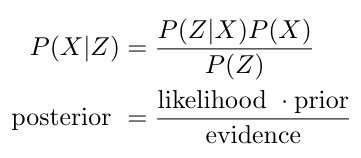
**I found it useful to see Bayes’ Theorem written out in words as follows [4]:

Equation 8

References:

[1] Brooks-Bartlett, J. “Probability concepts explained: Maximum likelihood estimation.” Towards Data Science on Medium. https://towardsdatascience.com/probability-concepts-explained-maximum-likelihood-estimation-c7b4342fdbb1 Visited 18 May 2020.

[2] Gallistel, C. R. “Bayes for Beginners: Probability and Likelihood.” Association for Psychological Science. https://www.psychologicalscience.org/observer/bayes-for-beginners-probability-and-likelihood Visited 18 May 2020.

[3] Wikipedia. “Likelihood function.” https://en.wikipedia.org/wiki/Likelihood_function Visited 06 May 2020.

[4] Balaban, J. “A Gentle Introduction to Maximum Likelihood Estimation.” Towards Data Science on Medium. https://towardsdatascience.com/a-gentle-introduction-to-maximum-likelihood-estimation-9fbff27ea12f Visited 18 May 2020.

[5] Gallistel, C. R. “Bayes for Beginners 3: The Prior in Probablistic Inference.” Association for Psychological Science. https://www.psychologicalscience.org/observer/bayes-for-beginners-3-the-prior-in-probabilistic-inference Visited 18 May 2020.

[6] Horii, S. “A Gentle Introduction to Maximum Likelihood Estimation and Maximum A Posteriori Estimation.” Towards Data Science on Medium. https://towardsdatascience.com/a-gentle-introduction-to-maximum-likelihood-estimation-and-maximum-a-posteriori-estimation-d7c318f9d22d Visited 18 May 2020.

[7] Wikipedia. “Conjugate prior.” https://en.wikipedia.org/wiki/Conjugate_prior Visited 18 May 2020.

[8] S, Y. “Maximum Likelihood Estimation VS Maximum A Posterior.” Towards Data Science on Medium. https://towardsdatascience.com/mle-vs-map-a989f423ae5c Visited 18 May 2020.

[9] Kim, A. “Conjugate Prior Explained.” Towards Data Science on Medium. https://towardsdatascience.com/conjugate-prior-explained-75957dc80bfb Visited 18 May 2020.