Although I have written a post on drawing Nyquist plots before, I was still feeling shaky in my understanding of the fundamentals, so I am going to use this post to try to cement my knowledge of where the Nyquist plot comes from. Please note that this entire explanation comes from Nise [1]; since this post is so detailed I am not going to cite specific sentences. Please understand that all information here comes exclusively from Nise [1].

Let’s start with what the Nyquist plot tells us and why we would use it. The Nyquist plot can be used to infer whether or not the closed loop version of a system is stable, based on knowledge of the open loop system. We use it to check for closed loop stability of a system, and to find the gain and phase margins of a system. Remember from earlier posts that it can be very difficult to analytically find the closed loop poles of a system without the use of a computer. The Nyquist plot sidesteps this challenge and helps us determine if any of the closed loop poles are in the right half plane, which indicates instability.

The important thing to clarify in this discussion is that there are some similarities and differences between the open loop and closed loop transfer functions for a system, and the Nyquist plot exploits these concepts. Consider the block diagram shown below, and write out the open loop transfer function in terms of the numerators and denominators for each transfer function in the block diagram.

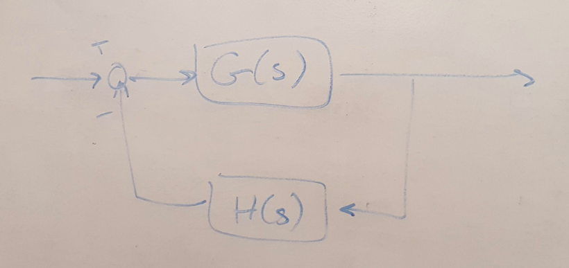Figure 1

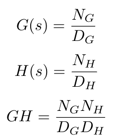
Now write out the characteristic equation for the closed loop system (i.e. 1 + GH) in these same terms. Do you see that the characteristic equation has the same poles as the open loop transfer function?

Now write the closed loop transfer function. Do you see that the zeros of the characteristic equation are equivalent to the poles of the closed loop transfer function?

These two key facts are going to be useful in a minute:

(1) The poles of the characteristic equation for a system are the same as the poles of the open loop system.

(2) The zeros of the characteristic equation are the same as the poles of the closed loop system.

Now let’s explore the idea of mapping contours. We can map complex numbers, s, through a function f(s) to obtain another complex number, w. Any function can be thought of as a map from one value to another. We can also map contours as a series of points through a function. A contour is any closed line that we can draw. Let’s get to used to thinking about mapping contours by reviewing some basic facts about them and drawing them out.

(a) If we draw a contour A in the clockwise (CW) direction, then the contour B (B is obtained from A after mapping through some function, F(s)) is also CW if:
(i) F(s) has only zeros
(ii) F(s) has poles NOT encircled by contour A. This fact is illustrated by cases 1-3.
(b) If contour A is CW, then contour B is CCW if contour A only encircles poles. This fact is illustrated by case 4.
(c) If contour A encircles a pole or a zero, then contour B encircles the origin.

I’ve drawn out 5 cases below to help illustrate this conceptually.

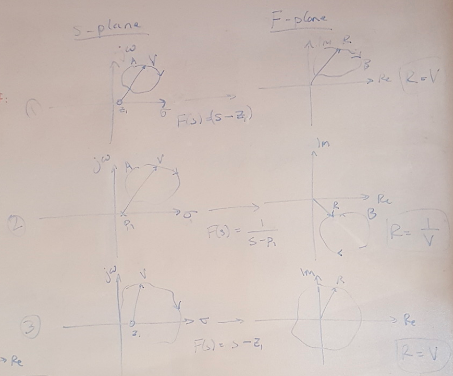Figure 2

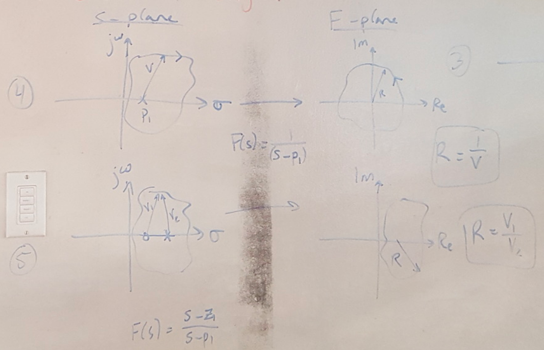Figure 3

I don’t think it’s necessary to memorize these facts, but I think the key takeaway is that the mapped contour B will look different depending on whether or not contour A contains poles or zeros. These facts will make sense if we next think about drawing a contour around the root locus plot. Let’s say that I have drawn a contour around the root locus and my mapping function is the characteristic equation, F(s) = 1 + GH. Then I can see that as I move CW around contour A:

(a) Every pole or zero inside the contour undergoes a 360 degree rotation.
(b) Every pole or zero outside the contour undergoes a net 0 degree rotation.
(c) A zero inside the contour contributes 360 degrees clockwise.
(d) A pole inside the contour contributes 360 degrees counterclockwise.

Figure 4

This is where I can get my Nyquist stability criterion from. From the observations above, I know that the net number of CCW encirclements about the origin, N, can be calculated as:

N = P - Z

Now let’s take one more step. As I mentioned at the top of this post, the characteristic equation, F(s) = 1 + GH, can be difficult for me to analyze because I may not be able to find the poles and zeros of the equation without the help of a computer. But it’s easy for me to find the poles and zeros of GH. So let me use GH as my mapping function, F(s) = GH. Recall that my equation above is looking for CCW encirclements about the origin, but now that I have defined a new mapping function, I want to find the number of CCW encirclements about -1, because:

1 + GH = 0

GH = -1

So here’s what I am going to do: I will draw a contour about the entire RHP of the root locus: I want to figure out if there are any poles in the RHP, because those will drive me to instability. Then I will map that contour using F(s) = GH and look for CCW encirclements abouts -1. I will use the same equation as before:

N = P - Z

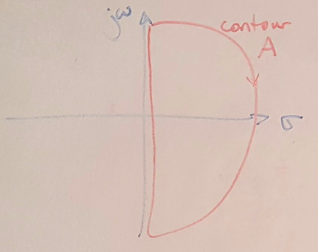Figure 5

Where N is the number of CCW encirclements of -1. P is the number of open loop poles in the RHP. We know from fact (1) above that this means that P is also the number of poles in the RHP for the characteristic equation. Therefore we can say that P is known because it is easy to find the RHP poles from the open loop transfer function. Z is the number of RHP zeros in the characteristic equation. From fact (2) above, we know that the zeros in the characteristic equation are also the poles of the closed loop transfer function. We do not know Z, so let’s rewrite the equation above:

Z = P - N

Now we can solve this expression. P is the number of open loop poles in the RHP and we can find this easily. N is just the number of encirclements of the Nyquist plot about -1, which is also easy to find. Then we calculate the value of Z. If Z is positive, then we know that we have unstable RHP closed loop poles, and therefore our closed loop system is unstable. I have two examples of this calculation below.

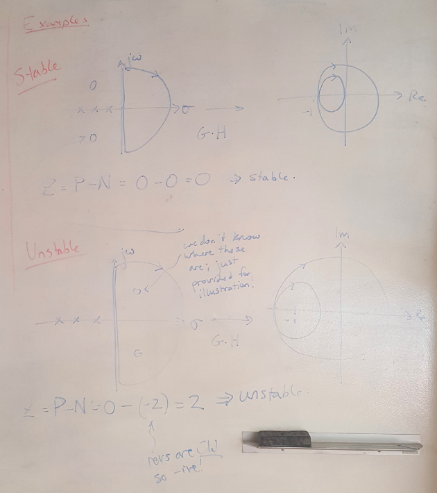Figure 6

References:

[1] Nise, Norman S. Control Systems Engineering, 4th Ed. John Wiley & Sons, Inc. 2004.