In this third and final post on filters, I want to explain how another kind of filter, the particle filter, works. We saw during our discussion of Kalman filters that they limit the user to thinking of the system as a Gaussian process, which may not be true in practice. The particle filter is a more general approach, and is popular in robotics and computer vision. If you want a brief, intuitive overview of the particle filter, I would strongly recommend watching this YouTube video by Uppsala University which is a fantastic explanation for what the particle filter is doing [1]. In this post, I will begin by laying out the framework of the particle filter, and then present the algorithm.

Framework for the Particle Filter

One of the key differences between the particle filter and the Kalman filter is that the particle filter can represent any arbitrary probability distribution, and that distribution does not have to be Gaussian [2,3]. We can do this by representing the probability distribution as a discrete collection of particles (or points), instead of as a continuous curve with an analytical expression [2,3]. This works nicely from a computational standpoint because we can just store information about all of the particles in a matrix. Each particle could be considered as its own hypothesis - each particle is a guess of what our state is at the current time step [2,3]. The particles can have weight, and that weight is correlated to how likely that particle is to be the true value of the state at the current time step [2,3].

Our objective is to iteratively update the distribution of particles so that eventually, the probability of choosing a particle from the distribution is equal to the probability that the system is truly at that state at the current time step [2]. In other words, you want the particles to be tightly concentrated around the true location of the robot. I represent that pictorially below in Figure 1. Consider a robot in a room, and the robot has a map of the room and a sensor that can collect measurements of the robot’s distance to the nearest solid surface in 360 degrees. Initially, at t = 0, the robot has no idea where it is. The distribution of particles is randomly distributed about the entire map. The robot moves forward by a known distance and takes a measurement. This measurement allows the robot to update the distribution of particles, and we can see that they cluster about a couple of locations where the robot could be located. This process repeats and in a few time steps, the robot’s particle distribution is tightly clustered about its current location. This is how the particle filter works.

Figure 1

When we use a particle filter, we will make some assumptions. The first is that we have a statistical model of our dynamic system and our actions - this is our prior belief about our system before we include our measurement data [2]. Secondly, we assume that our sensor model is the likelihood of getting a measurement, z, given state x, written as [2]:

Equation 1

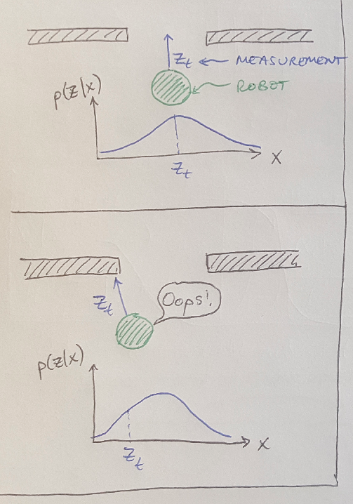
The concept of a likelihood is worth discussing here. (We previously touched upon it when we looked at VAEs.) The likelihood tells us how likely it is to get that measurement, z, if our state had the value x [2,3]. For example, let’s imagine we had a wall-following robot that had a sensor which told it whether it was in front of a wall or an open doorway, as illustrated in Figure 2 below [3]. If we were directly in front of an open doorway, the likelihood of detecting that open doorway is high [3]. However, if we were slightly off-center relative to the doorway, the likelihood of detecting the open doorway is reduced; our sensor might pick up the frame of the doorway and think we were in front of a wall instead [3]. This is what we mean by likelihood.

Figure 2 - Inspired by [3]

Our final assumption is that we now know our actions, u, at every time step [2]. (In control theory we call our actions our “control input.”) Now that we have some intuition for what our particle filter is doing, let’s look at the algorithm.

Particle Filter Algorithm

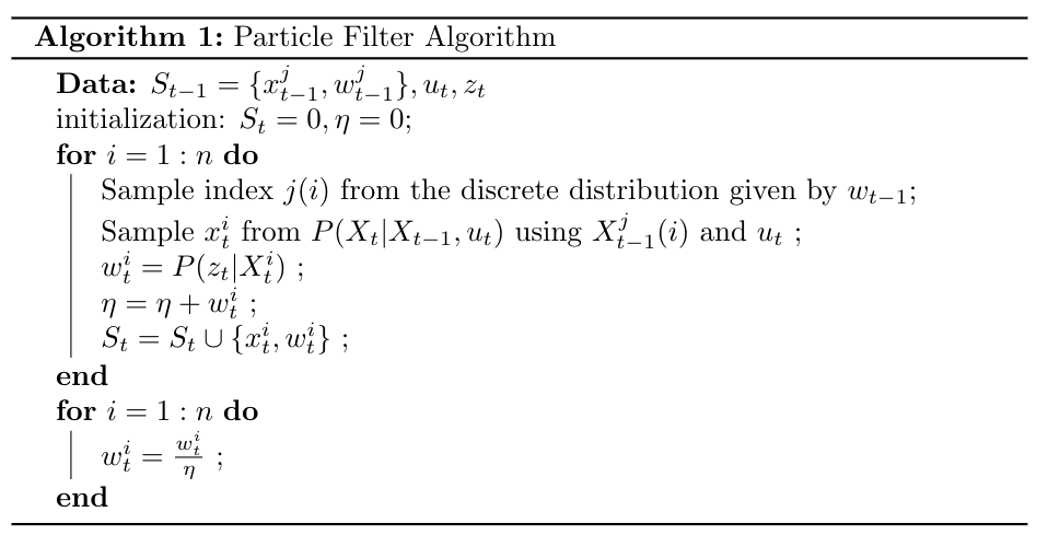
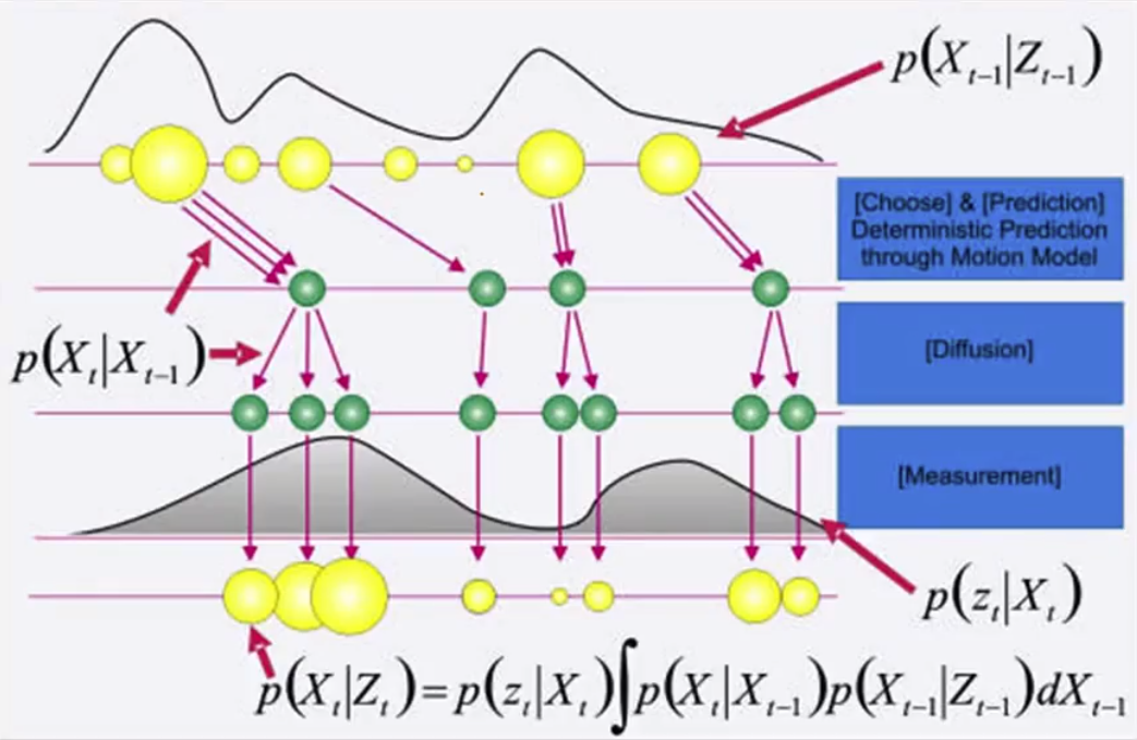
We present the particle filter algorithm below in Figure 3, and we’ll step through it using our wall-following robot again. A graphical representation of this conceptual process is also shown in Figure 4, and I will augment this discussion with images of the robot throughout the algorithm.

Figure 3 - Source [3]

Figure 4 - Source [3]

Initialization. We assume that at time t we have a prior probability, S, for our state at time t-1, x, and the weights of the particles representing the prior, w [3]. We also assume that we know our control input u and our measurement, z, for the current time step, t [3]. We are going to keep track of eta, which is a normalization factor that normalizes the weights so that they always sum to one (this is important because the weights are probabilities and the sum of the probability distribution is always one) [3].

Sampling. First we generate i samples (or particles) [3]. We pull the samples from the discrete distribution given by w from the previous time step, t-1 [3]. This is shown in Figure 5 below.

Figure 5

Control and diffusion. This step has two components to it [3]. First, my robot moves according to the control input, u [3]. This shifts all of my samples deterministically [3]. Notice that they don’t all move the same amount, because my actions have some uncertainty (see Figure 4) but the key point is that they all move and I know how much they move because I know my control input, u [3]. Then I need to account for the fact that there is some uncertainty in how my state changed (recall the stochastic drift from the Kalman filter) [3]. I can do this by adding noise to each sample that I drew [3]. Note that I add noise to the same particle, thereby multiplying the number of particles from that sample, according to how many times that particle was sampled before [3]. If you look at Figure 4, this means that when I sampled from the first yellow particle from the previous distribution 3 times, that tells me that I need to generate 3 new particles by adding noise to the sample 3 times [3]. This is representing the probability that I am at state x-t, given the probability that I was previously at state x-t-1 [3]. This should make sense intuitively - if there was a good chance that I was at a particular state x at t-1, then the probability that I am now at state x at t given that I was at state x-t-1 before is high.

Reweight. Now I have taken a measurement, and I use that data to update the weights of all my particles using the likelihood of that measurement [3]. This generates my new row of yellow particles in Figure 4. It also affects the density of all my particles as shown in Figure 6 [3]. The particles that represent a higher probability that I am really at that location are now bigger than the particles that have a lower probability of being the true state [3].

Figure 6

Update normalization factor. This is just a bookkeeping step - I need to add up all of my weights to get the normalization factor that ensures that the weights will add up to 1, since they represent probabilities [3].

Insert. Now I need to add my new prior distribution of particles to my set, S, so that I can use them for the next time step [3].

Normalize. Finally, I divide through all of my individual weights by the normalization factor [3]. This way, when I need to use the weights to drive the sampling of my prior, S, at the beginning of the next iteration of the algorithm, they will represent the probability of pulling a sample from each particle [3]. We can see the effect of the weights in Figure 7 which shows what the distribution of particles will be on the next time step, given how we adjusted the prior distribution on the last time step [3]. Notice that the particles have shifted to the right along with the robot [3].

Figure 7

Wrapping Up

Hopefully you can see that as we iterate through this algorithm, we will continuously tighten the distribution of particles until we are very certain of our current location. This wraps up our discussion of tracking and filtering, I hope you found it useful.

References:

[1] Svensson, A. “Particle Filter Explained without Equations.” Uppsala Universitat. 08 Oct 2013. https://www.youtube.com/watch?v=aUkBa1zMKv4 Visited 13 May 2020.

[2] Bobick, A. “Lesson 45: 7C-L1 Bayes filters.” Introduction to Computer Vision. Udacity. https://classroom.udacity.com/courses/ud810/lessons/3315558624/concepts/33205886160923 Visited 13 May 2020.

[3] Bobick, A. “Lesson 46: 7C-L2 Particle filters.” Introduction to Computer Vision. Udacity. https://www.youtube.com/watch?v=_LjBba2hnfk Visited 13 May 2020.