In this post about the MolGAN architecture [1], we will actually begin to explore another type of graph neural network architecture, the relational graph convolutional network (R-GCN) [2,3]. In the MolGAN architecture, both the discriminator and the reward function must process an input graph and return a scalar that evaluates whether the graph is real or fake (in the case of the discriminator) and if it successfully meets some design criteria (in the case of the reward function). Both the discriminator and the reward function use a relational graph convolutional network (R-GCN) [2, 3] to evaluate the input graphs. In this post, we will start to understand how R-GCNs work.

First we will present some fundamental concepts from graph theory that we need to understand how we can convolve a graph. Next, we will study how Kipf and Welling derived their approximation for convolution over a graph. In a follow-on post, we will look at how the ideas from spectral graph theory give rise to convolution for graphs, and then apply these ideas to R-GCNs.

Spectral Graph Theory

I’m going to solve the mystery right away and explain that the “spectral” in spectral graph theory refers to the “spectrum” of eigenvectors of a matrix that represents a graph, G [4]. But let’s figure out how we get there.

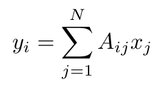
Previously I explained how we can describe the connections between nodes in a graph with an adjacency tensor, A. Let’s also represent the nodes in that graph as a single column vector, x, with N entries (where N is the number of nodes), and where each entry represents the value of each node [4]. If we multiply A and x together, what is the meaning of the result?

Equation 1

We can see that y is a sum of all the nodes that are connected to the i-th node [4]. There’s another way to write this equation, this time in terms of the eigenvalues and eigenvectors of this graph [4]:

Equation 2

Specifically, x contains the eigenvectors of the graph, and lambda represents the eigenvalues [4]. We can define the spectrum of the graph as a list of the eigenvectors of the graph, arranged in order of the magnitude of their corresponding eigenvalues [4]:

Equation 3

Thus the spectrum of a graph is a list of its eigenvectors arranged by magnitude.

There is one other concept that we need to introduce before we can move on. There is another matrix that we can write which describes the degree of every node, where the degree refers to the number of edges connected to a node [5]. The degree matrix, D, is diagonal, and every entry tells you the degree of the corresponding node [5]. We can use D to define the Laplacian matrix, L, as follows [5]:

Equation 4

The Laplacian is also an N x N matrix, and it is symmetric, just like A [5]. Note that every row and column sum to 0 in the Laplacian [5]. The Laplacian is going to play a central role in defining a graph and analyzing it.

Graph Propagation Function

Now that we have introduced the graph spectrum and the Laplacian, we are a step closer to understanding convolution over a graph. Before we dive into convolution, I just want to briefly introduce the idea of the graph propagation function [6]. This function will lead us to the graph convolution approximation used by Kipf and Welling in [3].

Specifically, we are looking for a propagation function that takes as input the adjacency matrix, A, and the node feature matrix, X, and returns some output Z at every node of the graph (the authors call z the output at the graph level after some pooling is done) [6]. We can define this nonlinear function as follows [6]:

Equation 5

Here, l refers to the number of layers in our network; H for the 0-th layer is X, and H for the L-th layer is Z [6]. Let’s consider a very simple example of a function, f( ), which could look like this [6]:

Equation 6

W is a weight matrix for the l-th layer, and sigma is some activation function like ReLU or tanh [6]. There are two small problems with this function. First, if we multiply with matrix A, for every node, we will add up all the features connected to it, but we will not include the features of the node in question [6]. So we need to add the identity matrix to A [6]. If this is confusing, consider the fact that the adjacency matrix has zeros along the diagonal - we add the identity matrix to change these values to one so that those nodes’ features are included in the summation over the rows during matrix multiplication.

The second problem with Equation 6 is that A is not normalized here, and so when we multiply X with A (when we are at layer 0), this will change the scale of the feature vectors of the nodes at that layer, and for every subsequent layer [6]. We can fix this problem by normalizing A so that all the rows sum to one, by applying the degree matrix, D [6]:

Equation 7

If you think about it, every row of A, which corresponds to one node, will be divided by its degree, so that the sum of the entries in that row sum to one. Equation 7 is essentially finding the average of the neighboring node features with respect to the node of interest [6]. Kipf suggests that it is more “interesting” if we rewrite Equation 7 as follows* [6]:

Equation 8

This now gives us a new expression for the propagation function, which can be written as [6]:

Equation 9

We use the tilde to indicate that we have added the identity matrix to A (i.e. A + I = A~) and D~ is the degree matrix of A~ [6].

Okay, now we have a graph propagation function over layers in our network. This function actually is our graph convolution function as well [3]. That’s right - Equation 9 is essentially a graph convolution function! But why? We can explain why Equation 9 is performing a first-order approximation of graph convolution by looking at the standard definition of convolution and manipulating it until we get an expression in the form of Equation 9 [3], which is exactly what we will do in the next post!

Footnotes:

*I honestly don’t understand why this is more “interesting” - if you have an idea, please let me know!

References:

[1] N. De Cao and T. Kipf, “MolGAN: An implicit generative model for small molecular graphs,” arXiv Prepr. arXiv 1805.11973, May 2018.

[2] M. Schlichtkrull, T. N. Kipf, P. Bloem, R. van den Berg, I. Titov, and M. Welling, “Modeling Relational Data with Graph Convolutional Networks,” in Lecture Notes in Computer Science (including subseries Lecture Notes in Artificial Intelligence and Lecture Notes in Bioinformatics), 2018, vol. 10843 LNCS, pp. 593–607.

[3] T. N. Kipf and M. Welling, “Semi-Supervised Classification with Graph Convolutional Networks,” 5th Int. Conf. Learn. Represent. ICLR 2017 - Conf. Track Proc., Sep. 2016.

[4] “Lecture 30 - THe Graph Laplacian Matrix (Advanced)

Stanford University.” YouTube. 12 Apr 2016. https://www.youtube.com/watch?v=FRZvgNvALJ4 Visited 28 Jul 2020.

[5] “4 9 Defining the Graph Laplacian 3 27 Advanced.” YouTube. 23 Jul 2016. https://www.youtube.com/watch?v=AR7iFxM-NkA Visited 28 Jul 2020.

[6] Kipf, T. “Graph Convolutional Networks.” 30 Sept 2016. http://tkipf.github.io/graph-convolutional-networks/ Visited 29 Jul 2020.