This post is a follow-on to my original introduction to drawing root locus plots. Last time we learned what a root locus is and how it can be drawn. Today I am going to focus on how we can derive useful information from the plot. Then I will close out this series with at least one more post on how we can then use root locus plots to design different kinds of controllers.

Let’s focus today’s discussion on a single example. The root locus equation is given below.

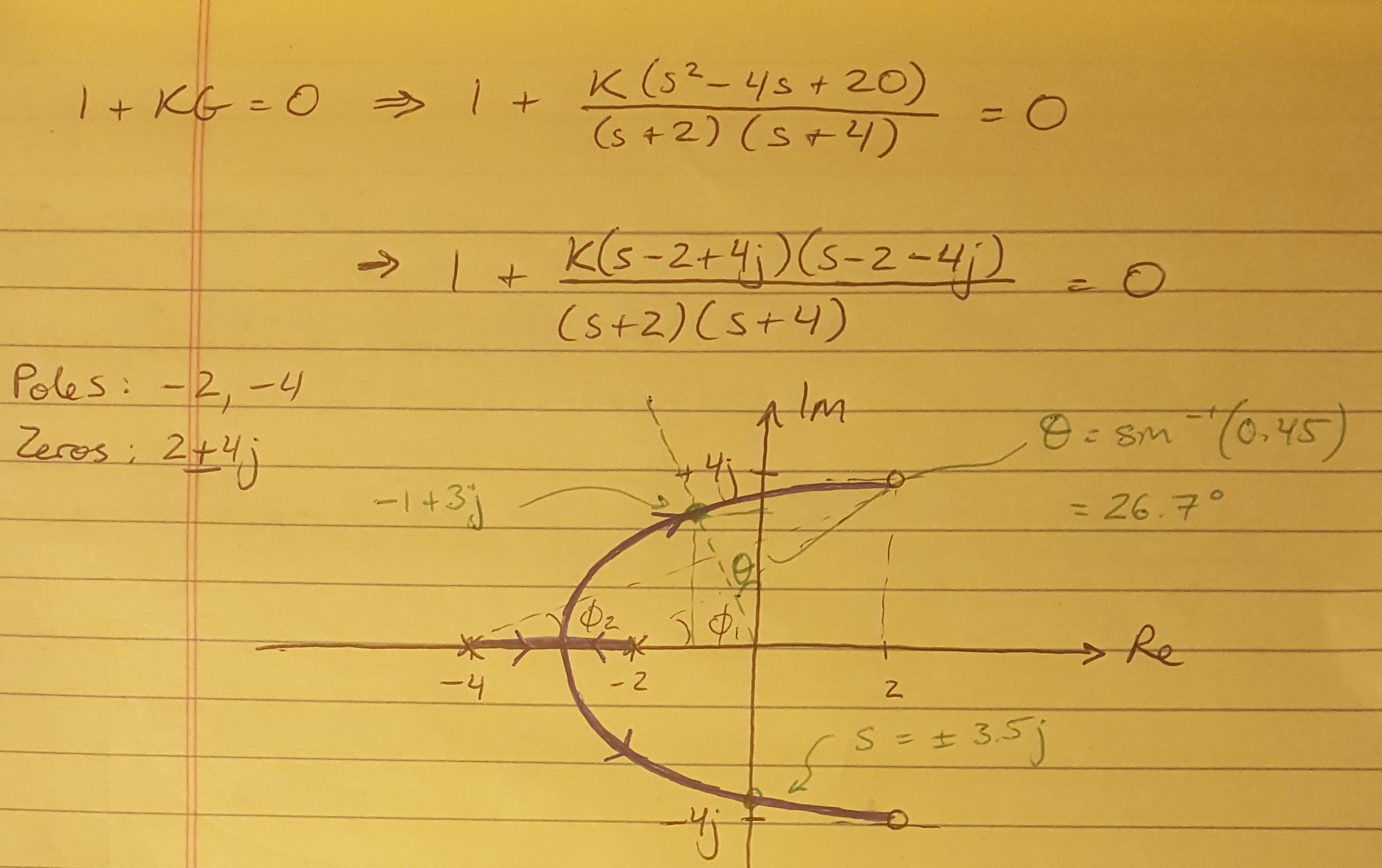
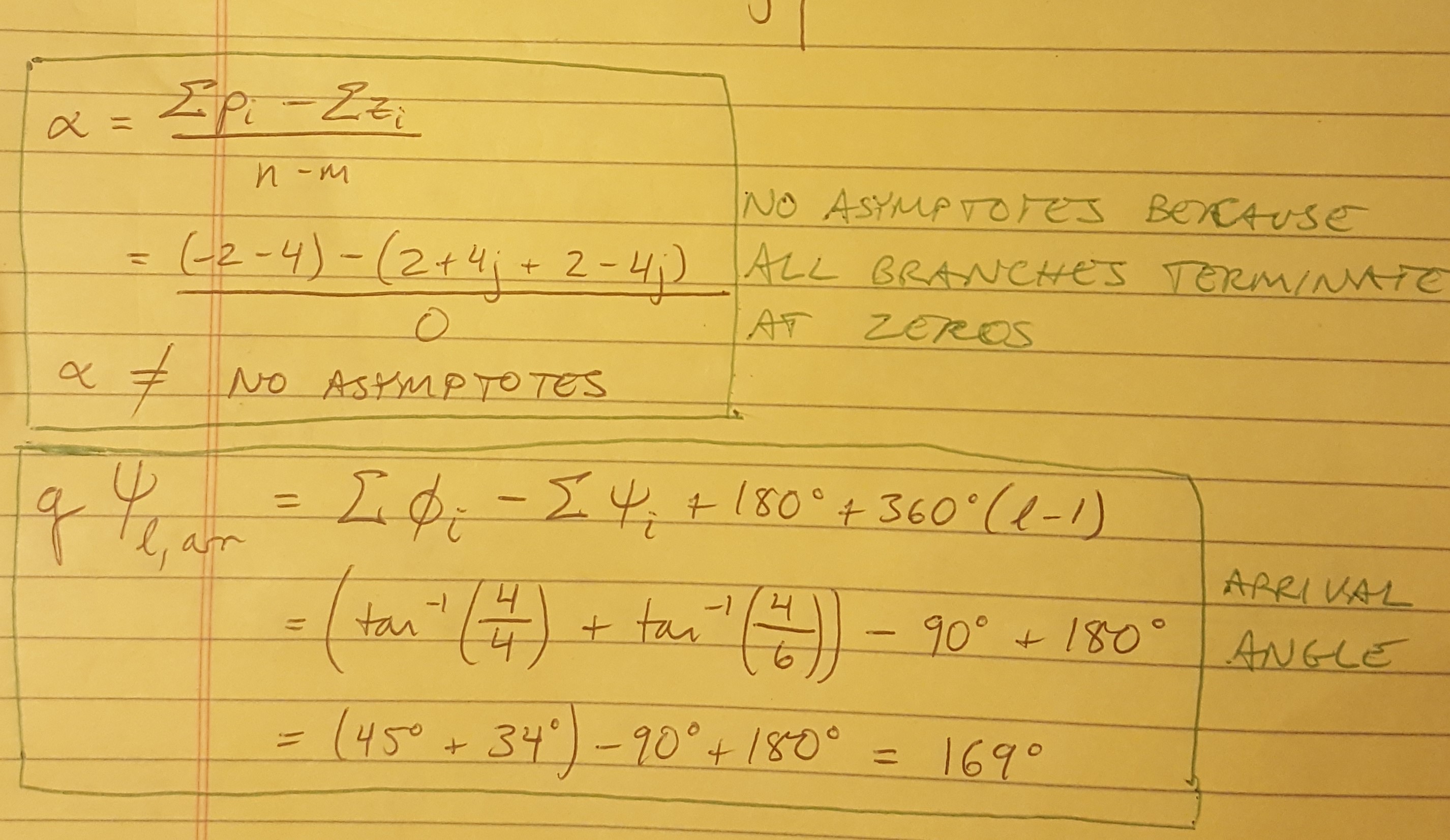
It has 2 poles and 2 zeros and the corresponding root locus is drawn in Figure 1. I should note that this example is copied from Example 8.7 in [1] and so I had a little help from the textbook to give me the correct shape of the root locus plot. My calculations for arrival angles are shown in Figure 2. You can see that I initially thought that I needed to calculate the position of an asymptote for the root locus, but when you have an equal number of poles and zeros, all the branches that originate from poles can terminate at zeros.

Figure 1

Figure 2

Now that we have the root locus drawn, let’s pause for a minute and discuss what information we can learn from it. First of all, the plot shows us the stability of the system. Any part of the root locus that is located in the right half of the plane is unstable. This is because a pole or zero in the right half plane has a time domain response that is wrapped in an envelope that can be expressed as a POSITIVE exponent of e, which INCREASES exponentially with time, thus resulting in instability (please refer back to Figure 1 in my previous post to see why this is). So if the locus crosses from the left to the right hand side, we should be able to tell what value of gain will drive the system unstable, or how additional poles and zeros (from a controller) could affect the system’s stability.

Figure 3

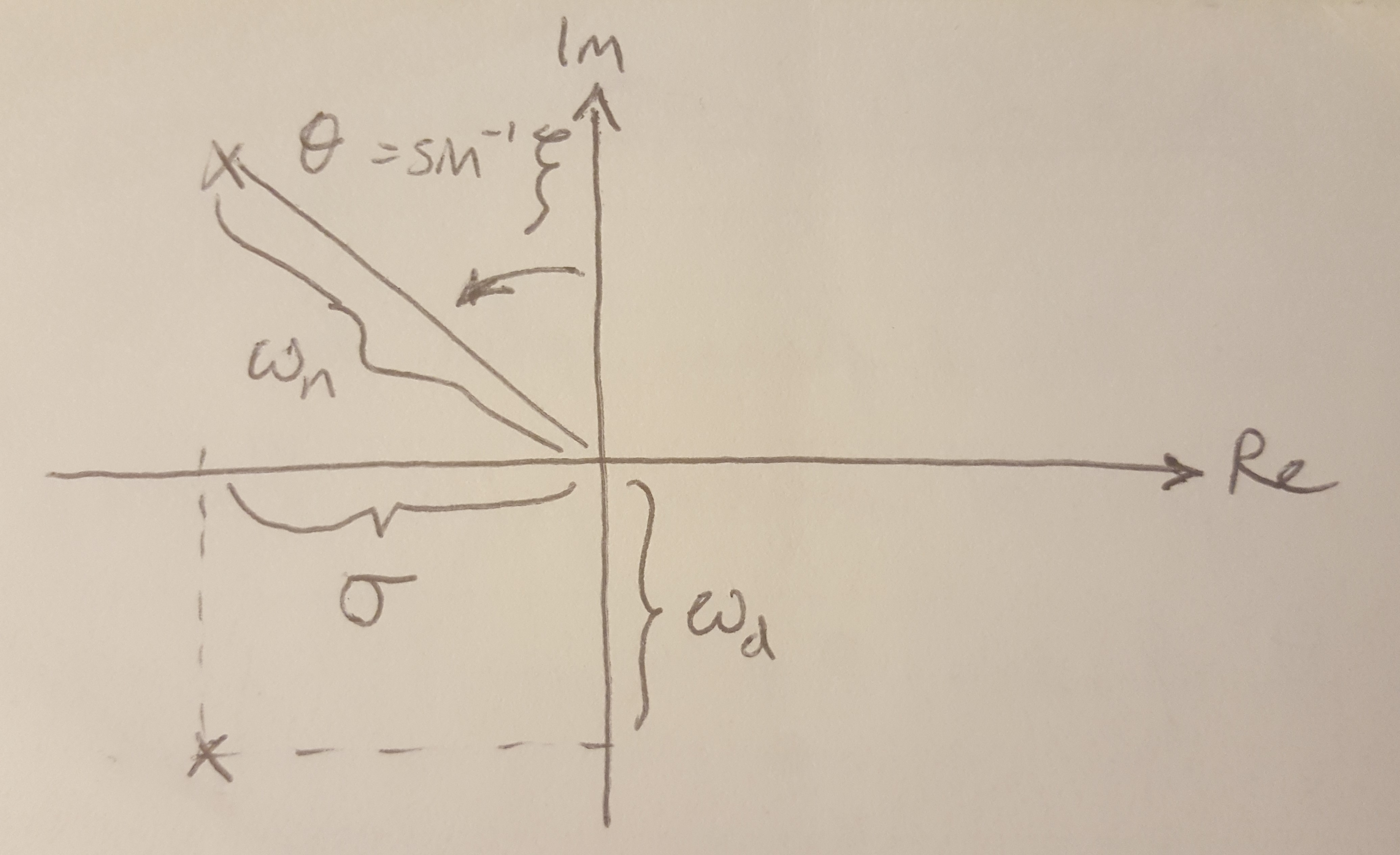
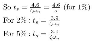
In Figure 3 I have provided a diagram showing how we can calculate some typical 2nd order time domain characteristics for the system at a particular point on the root locus. This shows us how we can find the natural and damped frequencies of the system for a given gain. We can also find a gain value that meets a desired damping coefficient. Once we have these basic values, we can go on to calculate other specifications of the 2nd order system that we might be trying to design to meet requirements, such as the peak time, rise time, settling time, overshoot and damping coefficient (based on an overshoot requirement). Those equations are shown below.

But remember that we are not always working with second order systems! These calculations will only be valid if you have a second order system or a good approximation of one. According to [1], a good approximation of a second order system can take several forms:

(1) The system has 2 poles close to the origin, and then additional poles and zeros are distant from these dominant poles ([1] recommends a factor of 5 distance away).

(2) The system has 2 poles close to the origin, as well as a zero in the vicinity. The zero is cancelled out by an additional pole that is relatively close to the zero, and therefore essentially negates its effect on the system.

Let’s return to Example 8.7 in [1]. Part of the question asks the student to find a gain that results in a damping coefficient of 0.45. Now, the textbook solves the problem with a computer program, but we can do an approximation of the solution by hand. First we can use the equation below to find that the angle corresponding to a damping coefficient of 0.45 is approximately 27 degrees. I draw a line that is 27 degrees from the Imaginary axis and find the point where it intersects the root locus, at s = -1 + 3j. Now go back to the root locus equation, 1 + KG(s) = 0, and plug in the value of s that we just found, and solve for K [2]. In this example, I found that the real part of K ~ 0.375 [3].

Similarly, I might also want to know what value of K will drive me to instability, so I can look for the locations on the Imaginary axis where the locus crosses over to the right half plane. Here I approximate the y-intercept as s = +/- 3.5j. Again, I can plug in my value of s into the root locus equation and solve for K, which I found to be K ~ 0.55.

References

[1] Nise, Norman S. Control Systems Engineering, 4th Ed. John Wiley & Sons, Inc. 2004.

[2] Douglas, Brian. “Root Locus Plot: Common Questions and Answers.” https://www.youtube.com/watch?v=WLBszzT0jp4&list=PLUMWjy5jgHK1NC52DXXrriwihVrYZKqjk&index=25&t=0s Visited 07/17/2019.

[3] Cheever, Erik. Linear Physical Systems Analysis, Department of Engineering, Swarthmore College. “Root Locus Examples.” https://lpsa.swarthmore.edu/Root_Locus/RLocusExamples.html Visited 07/17/2019.