In this second post on VAE’s, I am going to dive into the details of calculating the loss function. You will recall from my previous post that this is going to be more complicated than the loss function for a standard neural network because the variational autoencoder is learning to represent the latent space as Gaussian distribution [1].

The Loss Function for a VAE

Last time, we saw that the decoder can be presented as a function p(x given z) that reconstructs the output, x, from the latent space data, z [2]. The decoder is not necessarily going to do a perfect job of reconstructing x from z, so we can calculate the information lost using the log-likelihood function, or log( p( x given z ) ) [2]. There is a lot to unpack here, because likelihood, the log-likelihood, and the maximum likelihood estimate are big ideas that are useful all over machine learning. So I will direct the reader to this other post that just discusses likelihood, and for now we will focus on understanding how it pertains to the VAE. In a sentence, the likelihood function measures how well a statistical model fits to a sample of data; in other words, how likely the sample of data was to have come from the particular statistical model we are working with [3]. We can use the log-likelihood to write the loss function for a single data point as l - the total loss for N data points will just be the sum of the losses for each individual datapoint [2]. The loss function uses the negative log-likelihood function with a regularizer as follows [2]:

Equation 1

The first term represents the reconstruction loss (i.e. the error between what the decoder outputs and what the actual desired output was) [2]. The second term is a regularizer which we will discuss in more detail below [2]. First, let’s discuss the reconstruction loss. This is calculated as the expectation* of the negative log-likelihood of the i-th data point [2]. This term is encouraging the decoder to learn to accurately reconstruct the data [2]. If the decoder performs poorly, the log-likelihood function will show that the desired output has a very small chance of coming from the probability function represented by the decoder, p(x given z) [2]. Conversely, if the decoder is performing well, the log-likelihood function will indicate that there is a very good chance that the desired output came from the probability function p(x given z) [2].

Now let’s talk about what the regularizer is doing in the loss function. In general, in a variational autoencoder, we want the probability of z (i.e. p(z)) to be a normal distribution with mean of zero and a variance of one [2]. We can write this as p(z) = N(0,1) [2]. The encoder is learning to approximate this distribution with the function q( z given x) [2]. The regularizer will penalize the encoder if it chooses a function q(z given x) that is very different from a standard normal distribution [2]. Let’s represent this with an example. If we are trying to classify handwritten numbers written by different people, we would want the encoder to put a 3 written by Fatima in the same region of the latent space as a 3 written by Jorge [2]. This should make sense given that the point of latent space is to group similar input data together, and these 3’s written by Fatima and Jorge are, in principle, similar to one another [2]. However, if we did not have this regularizer in our loss function, the encoder might learn to cheat and just give every input data point its own, very distinct, representation in the latent space [2]. The latent space would grow to be very large and we would lose the benefit of having compressed all the input data into a smaller latent space. But since we do have a regularizer term, it will check that the encoder is building a latent space, described by z, that has a distribution similar to a normal distribution, and therefore the values of z are properly spaced in the latent space [2].

The regularizer in the equation above is called the Kullback-Leibler divergence [2]. The Kullback-Leibler (KL) divergence (also described as “relative entropy”) measures how different one probability distribution is from another [5]. If the KL divergence is 0, then it means that the two probability distributions are identical, and non-zero KL divergence values indicate that the two probability distributions are different [1]. We can write the KL divergence as follows [5]:

Equation 2

In other words, the KL divergence is an expectation (i.e. the weighted average) of the logarithmic difference between the two probabilities [5]. In our particular application, we will use the KL divergence to measure the difference between the ideal distribution of the values in the latent space, p(z), from the encoder’s learned distribution, q(z given x) [2].

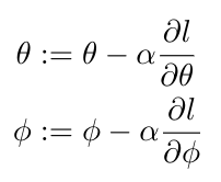
So now that we have a general understanding of the loss function, we can close the loop on how the VAE will learn. The encoder will take in the training data and compress it into the latent space, which is represented as a Gaussian distribution. The decoder will take a random sample from this latent space and output a data point that should be similar to the input. The loss function will check the performance of both the decoder and the encoder: it will check the decoder’s output to see how close it is to the desired output, and it will check the encoder’s learned distribution and make sure that it is close to a normal distribution. The loss function will inform the backpropagation algorithm which will be used to calculate the partial derivatives on all the nodes. We will use these partial derivatives to update the parameters of the encoder (theta) and decoder (phi) using gradient descent [2]:

Equation 3

Where alpha is the step size.

Bayesian Probability

We are now going to move away from thinking about VAEs as a neural network, and think about them in the context of probability. From a probability perspective, the encoder in the VAE is learning to infer** values of z, given observations of values of x [1,2]. We can use Bayes theorem to describe what the encoder is trying to do [1,2]:

Equation 4

We call p(z given x) the posterior distribution, because it is a distribution that we have calculated after taking a set of data, or evidence, into account [8]. In words, Bayes theorem describes the probability of an event based on our prior knowledge of some conditions that might be related to that event [7]. Just as an example of how Bayes theorem is useful, let’s say that we are using it to predict a person’s risk of a heart attack [7]. The chance of a heart attack increases with age [7]. By using Bayes’ theorem, we can calculate the probability of one person’s risk of heart attack by taking their age into account, which is a more accurate prediction than predicting one person’s risk of heart attack based solely on the distribution of risk over the entire population [7].

Let’s take another look at Bayes’ Theorem by rewriting the denominator [1]:

Equation 5

Basically, we can see that the denominator is the evidence, and we can calculate it by taking the sum over all the possible values of z - in other words, we have to consider all the situations where p(x) will exist [1,2]. This would literally take forever - it is what mathematicians call an “intractable problem” [1]. So to get around this challenge, we will approximate the posterior distribution [1,2]. This is a complicated process, involving more discussion of the KL divergence and a new concept, the Evidence Lower Bound, or ELBO [1,2]. I will pick up this discussion in my next post.

Footnotes:

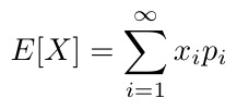
*The expectation in statistics is essentially the average of a lot of “independent realizations” of some random variable [4]. The expectation is different from an arithmetic average, though, because it takes into account the probability of each realization of the random variable [4]. Therefore we can say that the expectation is a weighted average of the independent realizations, where the weights of each realization are associated with the probability of that realization [4]. We can write it as follows [4]:

Equation 6

**In statistics and probability, we say that we are “inferring” something if we are using data analysis to figure out the properties of the probability distribution that produced the data we are analyzing [6]. One underlying assumption in this inference is that the data we are looking at is only a representative sample drawn from a larger population [6].

References:

[1] Stewart, M. “Comprehensive Introduction to Autoencoders.” 14 April, 2019. Medium: Towards Data Science. https://towardsdatascience.com/generating-images-with-autoencoders-77fd3a8dd368 Visited 24 March 2020.

[2] Altosaar, J. “Tutorial - What is a variational autoencoder?” https://jaan.io/what-is-variational-autoencoder-vae-tutorial/ Visited 06 May 2020.

[3] Wikipedia. “Likelihood function.” https://en.wikipedia.org/wiki/Likelihood_function Visited 06 May 2020.

[4] Wikipedia. “Expected value.” https://en.wikipedia.org/wiki/Expected_value Visited 06 May 2020.

[5] Wikipedia. “Kullback-Leibler divergence.” https://en.wikipedia.org/wiki/Kullback%E2%80%93Leibler_divergence Visited 06 May 2020.

[6] Wikipedia. “Statistical inference.” https://en.wikipedia.org/wiki/Statistical_inference Visited 06 May 2020.

[7] Wikipedia. “Bayes’ theorem.” https://en.wikipedia.org/wiki/Bayes%27_theorem Visited 06 May 2020.

[8] Stephanie. “Posterior Probability & the Posterior Distribution.” Statistics How To. 04 Mar 2016. https://www.statisticshowto.com/posterior-distribution-probability/ Visited 06 May 2020.