Welcome back to the blog. Today we are (still) talking about MolGAN, this time with a focus on the loss function used to train the entire architecture. De Cao and Kipf use a Wasserstein GAN (WGAN) to operate on graphs, and today we are going to understand what that means [1]. The WGAN was developed by another team of researchers, Arjovsky et al., in 2017, and it uses the Wasserstein distance to compute the loss function for training the GAN [2]. In this post, we will provide some motivation as to why we care about the WGAN, and then we will learn about the Wasserstein distance that puts the “w” in WGAN. Next, we will look at how the Wasserstein distance leads to the definition of a new loss function for the WGAN, and various implementations of this loss function. Our discussion closes with a comparison of the original WGAN with an updated version, the WGAN-GP.

Motivation

Before we get too far into this post, let’s stop and ask: why do we use the Wasserstein distance at all? Why isn’t a typical cost function with binary cross-entropy good enough? The problem with using binary cross-entropy to train a GAN is that, although it is generally a stable, effective approach for training the discriminator, it can be more difficult to train the generator with cross-entropy [4]. The reason why cross-entropy does not work so well is that the gradients that are used to train the generator can vanish if the generator’s fake samples are very far away from the real input [4].

Let’s consider this from an intuitive example. Let’s say that you are trying to guess a sound that your friend is imagining in their head, and the only thing they can tell you is if your guess is close or far from the sound they are imagining [7]. You have no idea what sound that might be, and there are a lot of possible sounds - maybe they are imagining a click, or a yodel, or middle C. If the sound they are imagining is a yodel, but your initial guesses are clicking sounds that you’re making with your tongue, your guess is so far from the truth that there is nothing similar between the clicking sound and the yodel. So they tell you that you are far from the truth, but that doesn’t help you guess what kinds of sounds will give you a better guess. It might take you a long time to try enough sounds before you make some kind of clicking sound that they say is close to the truth. This is an analogy for the vanishing gradient problem [7].

Okay, now let’s apply some formal mathematics to this idea. If we are using binary cross-entropy as our loss function, that means that we are using the Kullback-Leibler divergence as a metric of the difference between the true and approximated distributions, q(y) and p(y), respectively. We can plot the KL divergence as a function of the distance between the two distributions as shown in Figure 1, where we assume that the mean of q(y) is zero, and we vary the mean of p(y) [4]. This curve shows the farther p(y) is from q(y), the larger the divergence value, until it levels off at a maximum value [4]. This is the fundamental problem with vanishing gradients: if I am at point A in the plot, then the gradient of the KL divergence at this point is 0. The gradient is not telling me anything about how I should change the weights in my neural network to move p(y) closer to q(y). But if I were at point B, the gradient would be nonzero and it would give me information about how I need to change my approximation of p(y) to move it towards q(y). We are going to use the Wasserstein distance to address this problem [4].

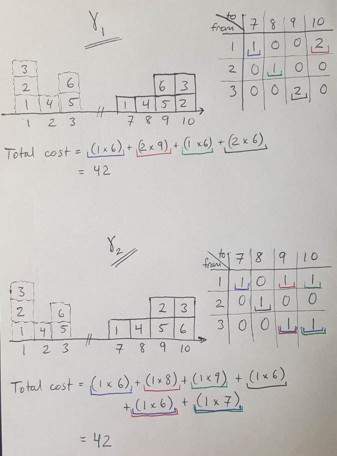
Figure 1 - Inspired by [4]

There are some other practical benefits to the WGAN that we cannot get from a traditional GAN. In his review of the Arjovsky et al. paper, Alex Irpan points out that the WGAN has some significant advantages over traditional GANs [13]. For example, you can train the discriminator to convergence in a WGAN, whereas in a vanilla GAN you are trying to balance the training of the discriminator with the generator, which can be a very sensitive process that is hard to repeat [13]. Secondly, the paper shows that the loss function for the generator actually correlates to the generator’s performance, which is not always true for traditional GANs [13].

Defining the Wasserstein Distance

We define the Wasserstein distance as the distance between two probability distributions [3]. It is sometimes referred to as the Earth mover’s distance because we can think of the Wasserstein distance in the following way: imagine we have two piles of dirt that represent two different probability distributions. The Earth mover’s distance is the cost associated with the amount of dirt we have to move to make the first pile look the same as the second [3]. Specifically, the cost is the product of the amount of dirt that has to be moved and the distance over which we have to move it. Note that it is possible for there to be more than one way to move the dirt from one pile to another; the Wasserstein distance is always the cheapest solution to this problem [4].

I want to briefly introduce another way to describe this problem discretely because it is useful for describing the mathematics below. In his Medium article, Hui explains that you can think of the Earth mover’s problem as a challenge to find the cheapest way to move a set of blocks from one configuration to another, as shown in Figure 2 [4]. The tables indicate two possible moving plans (which in this case have equal cost) [4].

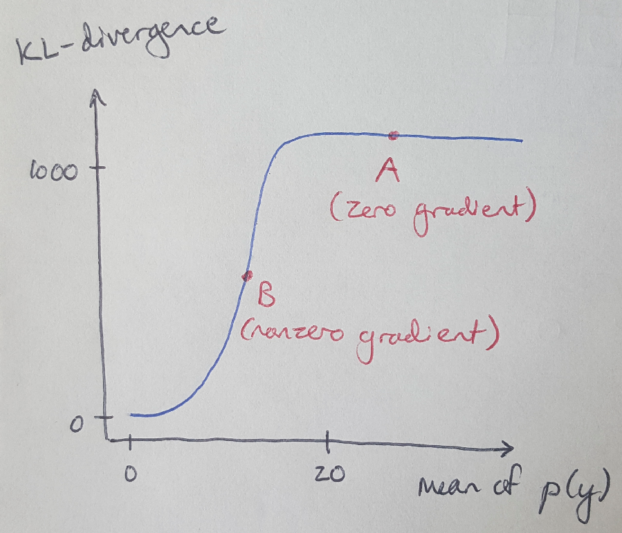
Figure 2 - Inspired by [4]

There is a formal mathematical definition for the Wasserstein distance, provided by Arjovsky et al. We can say that our current, or real, distribution is Pr, and the desired, or generated distribution is Pg [4]. The Wasserstein distance is the minimum cost transport plan [4]. We can also call this minimum cost the infimum, or the maximum value that is less than all the elements in a set - in our case, it is the maximum transport cost that is also less than all the other possible transport costs [4, 5]. The infimum is also called the greatest lower bound [5]. Mathematically, this can be written as [2, 4]:

Equation 1

Where Pi(Pr, Pg) is the set of all possible transport plans, gamma [4]. You could also say that Pi(Pr, Pg) is the set of all joint distributions that have marginal probabilities*1 Pr and Pg [2, 4]. Let’s return to our example in Figure 2 to explain how Equation 1 works.

We can choose values for x and y, where x is the starting location of a block and y is the final location of the block [4]. Then gamma(2, 7) is equal to the number of blocks that were moved from location 2 to location 7 along the number line [4]. That’s the value of the joint distribution for x = 2 and y= 7. Similarly, the sum of all blocks located at position y = 8 regardless of where they came from is equivalent to asking for the marginal distribution of y at position 8, or Pg at position 8 [4].

It is helpful to note that all of the blocks that we move from x must move to y [13]. That is, we cannot lose any mass from Pr as we are moving it to Pg [13]. This is why the marginal probabilities of Pi(Pr, Pg) must be Pr and Pg - the mass is conserved [13].

Now that we have a basic understanding of the Wasserstein distance, let’s use it to define a new cost function for the GAN that addresses the problem of vanishing gradients.

A New Cost Function

Let’s solve the mystery right away and show how the WGAN cost function performs relative to the vanilla GAN cost function. Consider Figure 3: we see the fake data distribution produced by the generator (green) is far from the real data distribution (dark blue) [2,4]. In this situation, a vanilla GAN cost function is shown in red. We can see that the red line has flat regions near the real and fake data distributions - in other words, the gradients are vanishing in this situation. In contrast, the WGAN cost function (cyan) has a nonzero slope everywhere. This is good news for us - even in this difficult setting, we have a nonzero gradient that can guide the weights in the generator’s neural network to improve its output.

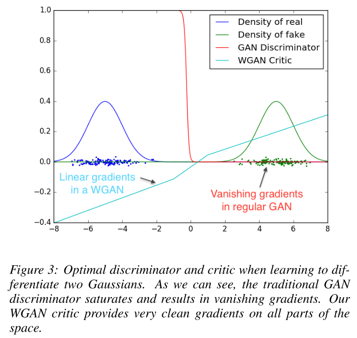
Figure 3 - Source: [2]

The only problem with computing the Wasserstein distance is that it is actually mathematically intractable to do so [4]. But that’s okay, we can reduce the calculation to make it simpler by using something called the Kantorovich-Rubinstein duality [4]. I promise to get into the mathematics of the Kantorovich-Rubinstein duality in another post, but just to keep things moving here I will not explain it here. Instead, I will wave my hands and give you the simplified version of the Wasserstein distance [4]:

Equation 2

Where theta is one single, real parameter [2]. The term sup refers to the supremum, which is the partner to the infimum: it is the smallest value that is greater than all the elements in a set [5]. The supremum is also called the least upper bound [5]. The function f is a 1-Lipschitz function which obeys the following constraint [4]:

Equation 3

I’m sorry but for efficiency’s sake I am also not going to explain Lipschitz functions here; I promise to write another blog post to address them.

Anyway, what we know now is that the Wasserstein distance can give us a better cost function than KL divergence. We know that we can write a simplified version of the Wasserstein distance using the Kantorovich-Rubinstein duality. And we know that this simplified expression requires us to use a Lipschitz function, f. Now we just need to learn what this function is; specifically, we can train a neural network to learn this function [4]. In fact, the discriminator is going to learn this function, f, with a few modifications [4]. First, the discriminator will no longer use the sigmoid function as its activation function, because the output logits will no longer represent probabilities - we are now going to ask the discriminator to return a scalar that represents a score [4]. The score defines how real the input images are [4]. Because of these modifications, Arjovsky et al. chose to rename the discriminator as the critic [2, 4]. Hui produced a nice graphic that highlights the differences between the GAN discriminator and the WGAN critic, as shown in Figure 4 [4].

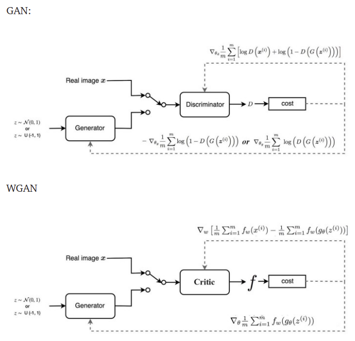
Figure 4 - Source: [4]

The bottom line is that the cost functions for the discriminator and the critic are different. We can write both as follows [4]:

Equation 4

We are almost ready to implement the WGAN and see how it performs in training. But before we do, there is one more thing that we need to implement to respect the constraint applied in Equation 3 [4]. We will see that enforcing this constraint can become problematic, and we will find a better alternative, in the next section.

Gradient Clipping and Alternatives

In Equation 3, we have bounded the value of the 1-Lipschitz function, and we need to build this constraint into our critic [4]. Arjovsky et al. used a gradient clipping approach to apply this constraint [2, 4]. This means that we restrict the weights of the critic, w, to be within some range defined by the hyperparameter, c, as follows [4]:

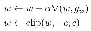
Equation 5

Arjovsky et al. used this gradient clipping scheme in their WGAN algorithm (which also trains the critic multiple times for every iteration of training of the generator) [2, 4]. They found that, although a typical GAN will show increasing generator loss even as the generator improves, the WGAN loss decreases, reflecting the improved accuracy of the generator’s outputs [2, 4].

The results presented by Arjovsky et al. are impressive and they show that the WGAN is much less likely to see mode collapse*2 than traditional GANs [2, 4]. They also show that the generator is able to train even when the discriminator is already performing very well - this would ordinarily be the kind of situation that produced vanishing gradients for a vanilla GAN [2, 4].

However, Arjovsky et al. are also willing to point out that the gradient clipping scheme they used to bound the 1-Lipschitz function was not an ideal solution [2, 4]. The training performance of the WGAN was highly dependent on the value of c: large values of c meant that it would either take a very long time for the weights of the critic to converge, or we would see exploding gradients (where the gradient of the loss function increases exponentially) [2, 4]. Similarly, small values of c led to the same problem of vanishing gradients that we saw before [2, 4]. This difficulty is shown in Figure 5 [9].

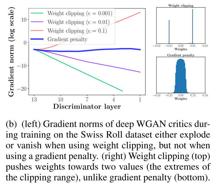
Figure 5 - Source: [9]

Another team of researchers, Gulrajani et al., investigated the problem of gradient clipping and found an improved method of bounding the 1-Lipschitz function [9]. The reason why gradient clipping was causing these instability issues, as illustrated in Figure 5, was that the gradient clipping was limiting the capacity of the critic to accurately model the 1-Lipschitz function [4]. If the model had more capacity, it could generate more complex boundaries that better fit the true distribution of the data [4]. This is illustrated in Figure 6, where Gulrajani et al. compared their alternative solution to the original WGAN and showed that their method was better able to generate contour lines that encompassed the model’s modes (the orange dots) [4, 9].

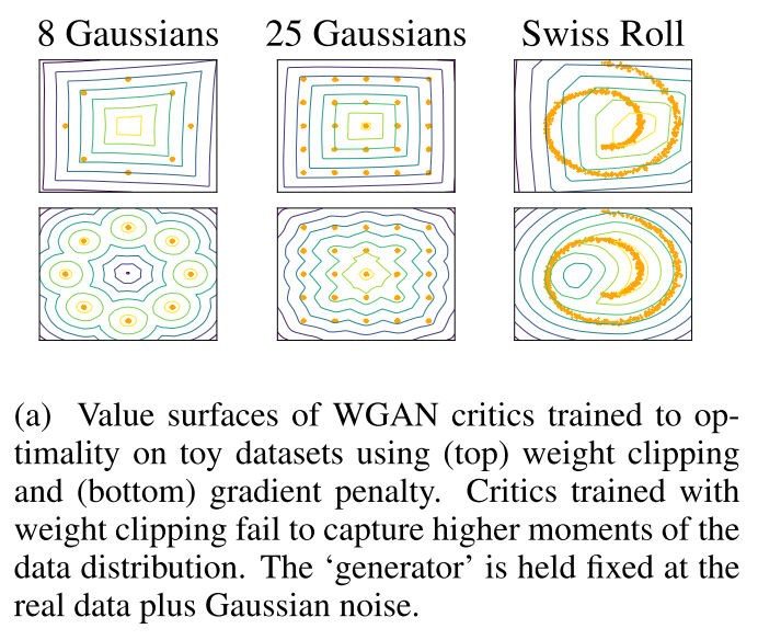
Figure 6 - Source: [9]

So what was Gulrajani et al.’s improvement to gradient clipping? They called their method a gradient penalty that ensures the critic approximates a 1-Lipschitz function by ensuring that the norm of the gradient of the function, f, does not exceed value 1 [4, 9]. So Gulrajani et al.’s WGAN-GP penalized the model if the gradient norm was far from 1 [4, 9]. We can write their loss function as follows [9]:

Equation 6

The authors set lambda to 10 throughout their work because they found empirically that this value performed well over different datasets [4, 9]. Also, a note on their implementation: they did not use batch normalization*3 for training the critic [4, 9]. This is because batch normalization can create relationships between samples in the same batch and this can affect the performance of the gradient penalty [4, 9].

In experiments, Gulrajani et al. showed that they had performance equal to a DCGAN baseline (a deep convolutional GAN) but that their WGAN-GP achieved a more stable inception score when it started to converge [4, 9]. The inception score*4 gives some indication as to how “realistic” the generator’s output is [12], so this result tells us that WGAN-GPs started to generate more reliably accurate images as it converged when compared to the DCGAN baseline. So even though the WGAN-GP does not clearly perform significantly better than the DCGAN, its improved reliability means that training the WGAN-GP will be more stable, which is always a good thing [4].

Conclusion

Hopefully this post has provided some clarity on what a WGAN is and how it differs from a traditional GAN. I would like to give lots of credit to Jonathan Hui’s posts on Medium, which were an excellent introduction to the WGAN and the starting point for this post [4, 8]. In my next post, I will go back and explain the Kantorovich-Rubinstein duality and the Lipschitz function in more detail.

Footnotes:

*1 Recall that marginal probabilities are the probabilities of an event, measured without taking into consideration the probability of other events in a set [6].

*2 Mode collapse is a phenomenon we see when training GANs, where the generator has learned to “cheat” by producing only a couple fake images that it has learned are very effective at beating the discriminator [8]. Mode collapse is undesirable because in this situation, the generator’s outputs are very limited, and we usually want a wide variety of outputs.

*3 Batch normalization is a method used to normalize the inputs to every layer in a deep neural network during mini-batch gradient descent [10, 11]. For example, given a mini-batch of data, we normalize the mini-batch (i.e. center the mean and adjust the scale, or variance, of the dataset) before it is fed to the neural network, and we also normalize the inputs to every hidden layer after the input layer in the network [10].

*4 The inception score is based on two criteria: (1) the images output by the GAN must be varied, and (2) each image must actually look similar to something real [12]. The inception score is high if both of these criteria are true [12]. The name “inception” comes from the “Inception” classifier network developed by Google, because the Inception classifier network can be used to obtain the inception score [12].

References:

[1] N. De Cao and T. Kipf, “MolGAN: An implicit generative model for small molecular graphs,” arXiv Prepr. arXiv 1805.11973, May 2018.

[2] M. Arjovsky, S. Chintala, and L. Bottou, “Wasserstein Generative Adversarial Networks,” arXiv Prepr. arXiv 1701.07875, Jul. 2017.

[3] “Wasserstein metric.” Wikipedia. https://en.wikipedia.org/wiki/Wasserstein_metric Visited 04 Aug 2020.

[4] Hui, J. “GAN - Wasserstein GAN & WGAN-GP.” Medium. 14 Jun 2018. https://medium.com/@jonathan_hui/gan-wasserstein-gan-wgan-gp-6a1a2aa1b490 Visited 04 Aug 2020.

[5] “Infimum and supremum.” Wikipedia. https://en.wikipedia.org/wiki/Infimum_and_supremum Visited 04 Aug 2020.

[6] “Marginal distribution.” Wikipedia. https://en.wikipedia.org/wiki/Marginal_distribution Visited 04 Aug 2020.

[7] Fry, H. “Life is like a game.” DeepMind: The Podcast. 20 Aug 2019. https://podcasts.google.com/feed/aHR0cHM6Ly9mZWVkcy5zaW1wbGVjYXN0LmNvbS9KVDZwYlBrZw/episode/MDNkOTllNzMtNTFlMy00YTQ1LWExYzgtMmZhMWM3ZmIzN2Rh?sa=X&ved=2ahUKEwiGoq2E7YHrAhUAg3IEHQSTBTgQkfYCegQIARAF Visited 04 Aug 2020.

[8] Hui, J. “GAN - Why it is so hard to train Generative Adversarial Networks!” Medium. 21 Jun 2018. https://medium.com/@jonathan_hui/gan-why-it-is-so-hard-to-train-generative-advisory-networks-819a86b3750b#4987 Visited 04 Aug 2020.

[9] I. Gulrajani, F. Ahmed, M. Arjovsky, V. Dumoulin, and A. Courville, “Improved Training of Wasserstein GANs.” arXiv Prepr. arXiv 1704.00028, Dec. 2017.

[10] “Batch normalization.” Wikipedia. https://en.wikipedia.org/wiki/Batch_normalization Visited 04 Aug 2020.

[11] Brownlee, J. “A Gentle Introduction to Mini-Batch Gradient Descent and How to Configure Batch Size.” Machine Learning Mastery. 21 Jul 2017. https://machinelearningmastery.com/gentle-introduction-mini-batch-gradient-descent-configure-batch-size Visited 04 Aug 2020.

[12] Mack, D. “A simple explanation of the Inception Score.” Octavian on Medium. 6 Mar 2019. https://medium.com/octavian-ai/a-simple-explanation-of-the-inception-score-372dff6a8c7a Visited 04 Aug 2020.

[13] Irpan, A. “Read-through: Wasserstein GAN.” Sorta Insightful. 22 Feb 2017. https://www.alexirpan.com/2017/02/22/wasserstein-gan.html Visited 04 Aug 2020.