I recently wrote a blog post about the backtracking approach to solving problems in computer science. Backtracking requires the use of recursion, which is another topic that I don’t know much about, so I’m going to use this post to explore the basics of recursion. We will talk about what it is and some basic examples of how to use it to solve problems.

The basic idea behind recursion is that we break a problem into smaller subproblems many times until the subproblem is so simple that we can directly solve it [1]. A simple example would be using recursion to solve the factorial problem, i.e. to calculate 5! [2]:

\(5! = 5 \cdot 4!\) – we write 5! as a product of 5 and 4!. Computing 4! is a subproblem of solving 5!
\(4! = 4 \cdot 3!\)
\(3! = 3 \cdot 2!\)
\(2! = 2 \cdot 1!\) \(1! = 1 \cdot 0!\)

We know that 0! is simply defined as the multiplication identity, i.e. 1, so now we have a subproblem that we can solve easily. We then work our way back up to compute 5! as follows [2]:

\(1! = 1 \cdot 1 = 1\)
\(2! = 2 \cdot 1 = 2\)
\(3! = 3 \cdot 2 = 6\)
\(4! = 4 \cdot 6 = 24\)
\(5! = 5 \cdot 24 = 120\)

The solution 0! = 1 is called the base case - this is the first case of the problem for which we know the answer by definition. The next case up in the recursion, 1!, is called the recursive case [2]. Notice that, in order for recursion to work, you must not only be able to break the problem into subproblems, but doing so must eventually lead to a base case [3]. There are certain instances where this would not happen (consider computing the factorial of a negative number), where we would never reach a base case, and in these situations, recursion cannot be used [3].

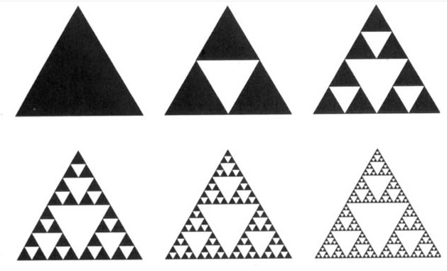
In the example used above, we solved one subproblem at each level of the recursive process. But it is possible to have multiple subproblems at one level - for example, when drawing a Sierpinski triangle, each level of the recursion requires splitting the 3 black triangles into 4 smaller triangles [4], as shown in Figure 1. For each level of the recursive algorithm, we are solving 3 subproblems instead of one.

Figure 1 - Source [5]

Efficiency of Recursive Algorithms

Recursive algorithms are not very efficient in terms of time. To see this in practice, let’s imagine we call a function to compute the factorial of 3 and 5. Within the function call factorial(3), we must call factorial(2) and factorial(1). For factorial(5), we have to call the factorial function 4 times, on {1, 2, 3, 4}. But we already have the values of the factorial function applied to {1, 2, 3} when we computed factorial(3), and it is time inefficient to repeat these computations [6].

One way to improve the efficiency of a recursive function is to use a technique called memoization. In this technique, we save the distinct outputs of our function calls in a table (also called the “memo” for memoization). So when we computed factorial(3), we would have saved the values for the factorial function applied to {1, 2, 3}. Then when we call factorial(5), we can first check our table to see if we already have the solutions to some of our subproblems and reuse them so that we speed up computational time. This technique is not necessarily space efficient, but as long as the memory required to store the table of values is not too expensive, it might be a useful way to speed up the algorithm in certain situations [6].

A second technique for speeding up recursion is to not use recursion at all, and replace it with a bottom-up approach. With this approach, we could compute Fibonacci numbers, fibonacci(n), as follows [6]:

• If n = 0 or n=1, return n
• Else repeat for n-2 times:
  • Initialize twoBehind = 0 and oneBehind = 1
  • Initialize result = 0
  • Compute result = twoBehind + oneBehind
  • Update twoBehind = oneBehind and oneBehind = result```
  • Return result

This approach requires performing far fewer function calls than a top-down, recursive approach and also requires much less memory [6]. Since this is obviously not a recursive algorithm, we call it instead an example of dynamic programming, which I plan to write about in more detail in a separate blog post [6].

As we’ve seen in the previous paragraphs, recursion can be a useful and elegant way to solve a problem, but it also has its drawbacks. Recursion is excellent for traversing trees, for example [7]. But, as discussed, recursion can be time (and space) inefficient. It can also be a confusing way to solve a problem, which you may want to avoid if your code is intended to be used by others [7].

Thank you for reading this post, I hope it was helpful. Next time we will talk about dynamic programming in more detail!

References

[1] “Recursion.” Khan Academy. https://www.khanacademy.org/computing/computer-science/algorithms/recursive-algorithms/a/recursion Visited 6 Jan 2022.

[2] “Recursive factorial.” Khan Academy. https://www.khanacademy.org/computing/computer-science/algorithms/recursive-algorithms/a/recursive-factorial Visited 6 Jan 2022.

[3] “Properties of recursive algorithms.” Khan Academy. https://www.khanacademy.org/computing/computer-science/algorithms/recursive-algorithms/a/properties-of-recursive-algorithms Visited 6 Jan 2022.

[4] “Multiple recursion with the Sierpinski gasket.” Khan Academy. https://www.khanacademy.org/computing/computer-science/algorithms/recursive-algorithms/a/the-sierpinksi-gasket Visited 6 Jan 2022.

[5] Qualman, D. “Sierpinski gasket or triangle fractal collapse.” https://www.darrinqualman.com/fractal-collapse/sierpinski-gasket-or-triangle-fractal-collapse/ Visited 6 Jan 2022.

[6] “Improving efficiency of recursive functions.” Khan Academy. https://www.khanacademy.org/computing/computer-science/algorithms/recursive-algorithms/a/improving-efficiency-of-recursive-functions Visited 11 Jan 2022.

[7] Sturtz, J. “Recursion in Python: An Introduction.” Real Python. 10 May 2021. https://realpython.com/python-recursion/ Visited 11 Jan 2022.