This is the third post in a series on graph networks, based on a recent paper by researchers at DeepMind [1]. So far we have discussed the motivation for why graph networks are useful for advancing AI research, and how they work from a probability perspective. Now I am going to briefly explain how the structure of a graph is useful in learning to model real-world processes, and present some of the mathematical framework for how graph networks learn.

Distributed Representations and Isomorphism

Graphs represent entities and relations as distributed representations [1]. That is, they can represent many different entities by using unique combinations of a fixed number of features [2]. I did not really understand this until I read a post by Ganesh which had an excellent diagram representing the idea of distributed representation, which is recreated below as Figure 1 [2]. As the right column of this diagram shows, the idea behind distributed representation is that we can, for example, describe many different shapes using a combination of features [2]. The first shape can be described by the features “vertical” and “rectangle” [2]. The second shape is also a “rectangle” but it is “horizontal” instead of vertical [2]. In contrast, a non-distributed representation assigns a unique label to every new shape that we need to represent, as shown in the left column of Figure 1 [2]. The great advantage of distributed representation is that I could conceivably represent an infinite number of different entities with the same defined set of features [2]. Moreover, I can compare different shapes by comparing which features they have in common, and which features they have that are unique - my non-distributed representation does not allow me to do that [2]. This idea is very powerful in graph networks because it adds to the graph’s ability to reason about the real-world situation that it is trying to model.

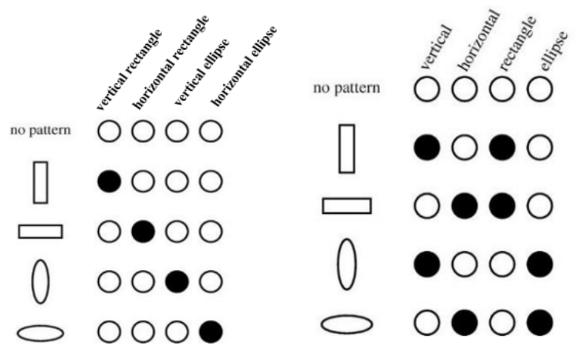
Figure 1 - Source [2]

There are many different ways to structure a group of entities in a graph. Perhaps the simplest method is a fully connected layer (think back to our discussion of neural networks, where every node in one layer is connected to every node in the previous layer and the next layer) [1]. In this structure, the entities are the nodes in the network, the relations are between every node in every layer and the rules are defined by the biases and the weights in each layer [1]. We say that the fully connected layer has a “weak relational inductive bias” because it does not enforce a lot of bias - any node can talk to any other node in the adjoining layers [1].

One advantage to using a graph is that it can represent a set of entities, where the order does not matter [1]. For example, we may want to use a graph network to learn the mass of a solar system given n planets [1]. In this situation, the order in which we add up the masses of all the planets should not matter, and so in this case, we say that we would like our approach to be “invariant to ordering” [1]. If we were not using a graph - instead let’s say we were using a standard neural network that processes a vector of data - then the neural network might return different total masses for the solar system when the input data is presented in different orders, even though the order in which the data is given should not matter [1]. The power of a graph network is that the graph representation does not care about the order of the nodes, so we do achieve the goal of ordering invariance [1].

A quick note about order invariance with graphs: just as the order that the nodes are listed should not matter in a graph, neither should the configuration of the graph matter, as long as different configurations are isomorphic [1]. Two graphs are said to be isomorphic if they have the same number of vertices, edges and the same configuration of edge connections [3]. Consider Figure 2 below - graphs G1 and G2 are isomorphic because they have the same number of vertices and edges, and the same vertices are connected in the same way [3]. In all the ways that matter, these graphs will both function the same in a graph network.

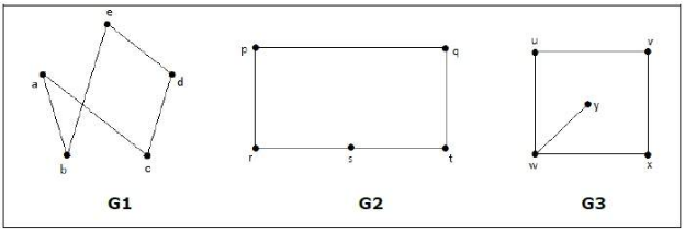
Figure 2 - Source [3]

Another advantage of using a graph is that it allows us to consider relations between arbitrary groups of nodes. Let’s imagine we are trying to model the motion of planets in a solar system, which requires considering the pairwise gravitational interactions between the planets [1]. We could do this without a graph, by computing the state of each planet as a function, g, of the force induced by the j-th planet on the i-th planet. The drawback to this approach is that the same function g would be applied everywhere (we call this “global permutation invariance”), which we may not want if the interactions between some planets were different from others. This approach does have an advantage in that it can, at least, support some kind of relational structure because it will consider two planets at a time. You could extend this function to consider nearest neighbors, or to consider all the planets (which would look like a fully connected layer).

We just considered two relational structures: no relations (to calculate the mass of a solar system) or all pairwise relations (to calculate the positions of the planets in the solar system). But many real-world systems are somewhere in between these two examples; sometimes the relations are not consistent between all nodes. What can we do to capture this situation? We would need a graph network where we can define where the relations between entities do exist, and where they don’t [1]. Let’s examine how a basic graph network operates.

Basic Graph Network Framework

The DeepMind paper states that the graph network framework “defines a class of functions for relational reasoning over graph-structured representations” [1].* The graph network (GN) block is the main computing unit in their framework: by definition, it takes in a graph as input, performs computations on it, and returns another graph as output [1]. The key design principles for a GN block are (1) that it allows for flexible representations, (2) it has a configurable within-block structure and (3) it can be composed into multiblock architectures [1]. Their definition represents the GN block as a directed, attributed (i.e. the nodes and edges have attributes) multigraph (i.e. it has multiple edges) with global attributes (i.e. attributes that describe the entire graph) [1].

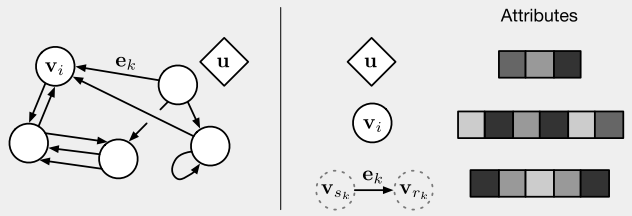
Figure 3 - Source [1]

The nodes are represented as v_i, the edges as e_k, and the global attributes are u. We can consider every edge as having a sender node (v_sk) and a receiver node (v_rk) (defined by the direction of the edge), as shown in Figure 3 [1]. In general, a GN block will first update (1) the edges, then (2) the nodes, and then (3) the global attributes [1]. The update algorithm is shown in Figure 4, and the general process is illustrated in Figure 5. The GN block will use update functions, phi, to map updates to all of the edges, nodes and global features [1]. The update functions will update each element individually [1]. A second set of functions, rho, will aggregate all of the updates for each node and edge [1]. The aggregator functions must be invariant to the input, no matter what permutation it is given as, and it must accept a variable number of arguments [1]. An example of an aggregator function is element-wise summation [1].

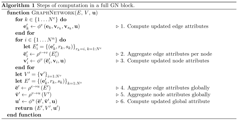
Figure 4 - Source [1]

Figure 5 - Source [1]

We can formally define the update functions as follows [1]:

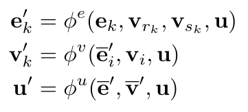
Equation 1

And the aggregator functions as [1]:

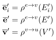
Equation 2

Where we define the nodes and edges as follows [1]:

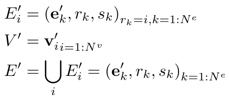
Equation 3

We can describe the computation steps as follows, imagining that we are updating the positions of a group of balls connected by springs [1]:

(1) Update all of the edges (akin to calculating forces or potential energy between two connected balls).

(2) Aggregate all of the edge updates (sum all the forces and energy on the i-th ball).

(3) Update all of the nodes (calculate new positions, velocities, energies for each ball).

(4) Aggregate all edge updates for use in the global updates (sum the forces and potential energies for all of the balls).

(5) Aggregate all node updates (calculate total kinetic energy of the system).

(6) Update the global attributes (calculate net forces and total energy of the system).

With that, I will end this series of posts on graph networks. I would definitely encourage the reader to look at the DeepMind paper for themselves, it is an excellent read and I only scratched the surface of what it discussed [1]. Thank you for reading!

Footnotes:

*Notice that the DeepMind paper does not use the word “neural” in their description of graph networks. The reason for this is that they are trying to generalize their framework - while you could use neural networks to represent the functions, it is not mandatory [1]. However, the authors do note that they use neural networks in their implementation of sample code, available on Github [1,4].

References:

[1] P. W. Battaglia et al., “Relational inductive biases, deep learning, and graph networks,” Jun. 2018. ArXiv ID: 1806.01261. https://arxiv.org/abs/1806.01261

[2] Ganesh, P. “Distributed Vector Representation: Simplified.” Towards Data Science on Medium. 14 Oct 2019. https://towardsdatascience.com/distributed-vector-representation-simplified-55bd2965333e Visited 08 May 2020.

[3] “Graph Theory - Isomorphism.” TutorialsPoint. https://www.tutorialspoint.com/graph_theory/graph_theory_isomorphism.htm Visited 08 May 2020.

[4] Graph Nets library. Github. https://github.com/deepmind/graph_nets Visited 12 May 2020.