I have been meaning to write this post about the Gumbel-softmax distribution for several months, but I put it on a back burner after I had dug myself into a hole of deep confusion and couldn’t get out. After some encouragement from my advisor, I decided to pick it up again, and this time I think I was able to figure things out.*1 So in this post, we are going to learn how the Gumbel-softmax distribution can be used to incorporate categorical distributions into algorithms that use neural networks and still allow for optimization via backpropagation [1, 2].

First we will discuss why it is difficult to work with categorical distributions, and then we will build up the Gumbel-softmax distribution from the Reparameterization Trick and the Gumbel-Max trick.

Why Is This Hard?

The problem that we will address in this post is how to work with discrete data generated from a categorical distribution [1-4]. A categorical distribution is a probability distribution made up of discrete categories [5]. For example, let’s draw inspiration from the MolGAN work and think about generating graphs that represent molecules. We can limit ourselves to generating graphs that only contain carbon (C), oxygen (O) and fluorine (F) atoms. In this situation, we will have a categorical distribution of the probabilities of choosing each atom type for each node in our graph. This idea is shown in Figure 1.

Figure 1

Now let’s say that I have a neural network that is going to output samples, z, pulled from this categorical distribution of atoms. These samples, z, will represent the atoms in my generated molecule. During the forward pass, the nodes in the final layer of my neural network return these samples. But when I need to optimize my neural network via backpropagation, I will not be able to compute the gradient across these nodes [1-4]. This is because these nodes represent a stochastic process defined by a discrete distribution, and it is impossible to compute a smooth gradient for either a stochastic or discrete process [1-4]. So I need to find another way to generate graphs that will allow me to perform backpropagation.

The Reparameterization Trick

The first thing I am going to do is apply the Reparameterization Trick. We have talked about it before but I’m going to briefly repeat it here. Let’s imagine for a moment that I have a continuous distribution of atoms that I can draw samples from, instead of a categorical distribution. (I know that doesn’t really make sense physically, but bear with me.) Imagining my distribution of atoms as continuous solves one of my problems, because now I don’t have to take the gradient of a discrete process. But how do I deal with the stochasticity of the sampling process?

We use the Reparameterization Trick to recast the stochastic sampling process as a linear combination of a deterministic and a stochastic element [1-4]. In other words, instead of saying that the nodes in the final layer of my neural network are directly sampling from the continuous distribution (which is a completely stochastic process), I can say that the nodes in the final layer are a linear combination of two nodes in the previous layer [1-4]. Specifically, I can say that the samples, z, come from a sum of the mean of the distribution plus some stochastic noise [1-4]. Why is this better? Because now I can directly compute the gradient of the mean and the variance of the continuous distribution, and I can bypass the stochastic node completely [1-4]. I illustrate this in Figure 2 and also give some equations below to help demonstrate what I’m talking about [1-4]:

Equation 1

Note that the noise we are adding is white noise centered about the zero-mean, so it does not add bias to our samples.

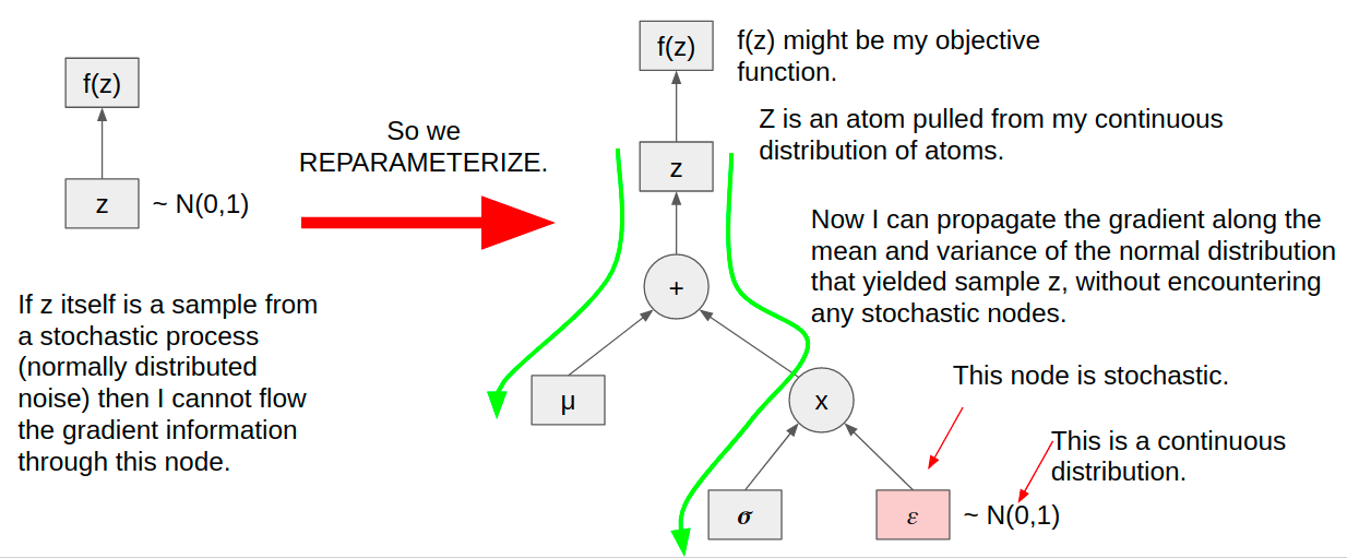
Figure 2 - Inspired by [1, 3]

Okay, so now I have a way of dividing a sampling process into separate deterministic and stochastic components. However, I did ask you to temporarily imagine that our distribution of atoms was continuous, and of course that’s not actually true. So how can we draw samples from a discrete distribution instead of a continuous one? That’s where the Gumbel-Max Trick comes in.

The Gumbel-Max Trick

The Gumbel-Max Trick was introduced a couple years prior to the Gumbel-softmax distribution, also by DeepMind researchers [6]. The value of the Gumbel-Max Trick is that it allows for sampling from a categorical distribution during the forward pass through a neural network [1-4, 6]. Let’s see how it works by following Figure 3.

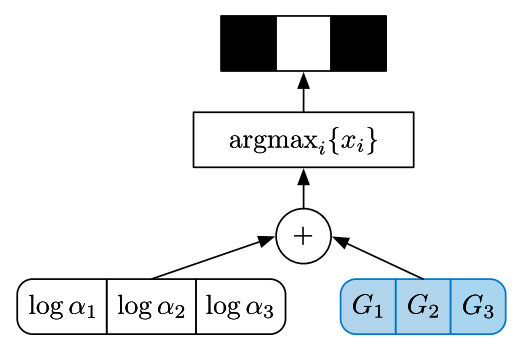
Figure 3 - Source: [2]

First, the Gumbel-Max Trick uses the approach from the Reparameterization Trick to separate out the deterministic and stochastic parts of the sampling process [1-4,6]. We do this by computing the log probabilities of all the classes in the distribution (deterministic) and adding them to some noise (stochastic) [1-4,6]. In this case, we use noise generated from the Gumbel distribution, which I will discuss more in a minute [1-4,6]. This step is similar to that used in the Reparametrization Trick above where we add the normally distributed noise to the mean.

Once we have combined the deterministic and stochastic parts of the sampling process, we use the argmax function to find the class that has the maximum value for each sample [1-4,6]. The class (or sample, z) is encoded as a one-hot vector for use by the rest of the neural network [1-4,6].

So now we can see that the Gumbel-Max Trick is very similar to the Reparameterization Trick, but we are adding the argmax function to it, and using noise sampled from a different kind of distribution. In fact, why are we using the Gumbel distribution to generate the noise here? An exact mathematical explanation escapes me, but I know that the Gumbel distribution is typically used to model the distribution of the maximums for a number of samples pulled from other distributions [7]. For example, if you wanted to predict which month in 2020 the Monongahela River will flood, the Gumbel distribution could be used to model monthly river level data over the past 10 years and thus extrapolate which month in 2020 will have the highest water levels [7]. Since the Gumbel distribution is used to model the distribution of maximums, it makes sense to me that Maddison et al. explained the selection of the Gumbel distribution by stating that it “is stable under max operations” [2].

One final note on this point - there is also a mathematical proof available that proves the Gumbel-Max Trick is equivalent to computing the softmax over a set of stochastically sampled points.

Bringing It All Together

We now have almost all of the pieces of the puzzle assembled. We have a way to separate the stochastic from the deterministic in the sampling process, and we have provided a means for sampling from a categorical distribution, as opposed to a continuous distribution. However, the argmax function in the Gumbel-Max Trick is not differentiable [1-4, 6]. So can we replace the argmax function with something that is differentiable?

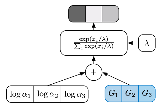
Figure 4 - Source: [2]

In fact you can, and both [1] and [2] proposed using the softmax function as a replacement for the argmax function, as demonstrated in Figure 4 [1-4]. In this approach, we still combine the log probabilities with Gumbel noise, but now we take the softmax over the samples instead of the argmax. Both groups also added a temperature factor, defined by lambda, which allows us to control how closely the Gumbel-softmax distribution approximates the categorical distribution [1-4]. This modified softmax function can be written as follows [1-4]:

Equation 2

Notice that I am following Jang’s convention of using y to denote “a differentiable proxy of the corresponding discrete sample, z” [1].

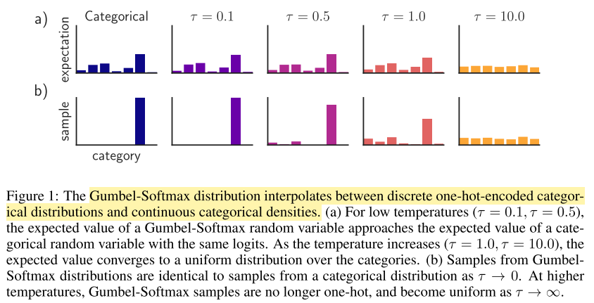
Figure 5 - Source: [1]

Let’s see how the temperature factor, lambda, can affect the shape of the Gumbel-softmax distribution. In Figure 5, we see Jang et al.’s presentation of how the Gumbel-softmax distribution becomes more uniformly distributed as the temperature increases [1]. In Figure 6, Maddison et al. also show how increasing the temperature shifts the distribution of probabilities to be uniformly distributed between all classes of the discrete distribution [2]. I like Figure 6 because it also gives us a visual example of what a simplex*2 looks like, since a 2-dimensional simplex is, in fact, a triangle [8]. We can see that for zero temperature, the distribution is discrete, and the probability of choosing one of the classes is concentrated at the vertices of the simplex [2]. As the temperature increases, the probability density is redistributed gradually until it is more centered in the middle of the simplex [2]. For more intuition about the effect of the temperature on the Gumbel-softmax distribution, Eric Jang has a fantastic interactive model on his personal blog.

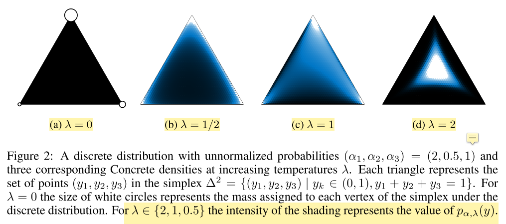
Figure 6 - Source: [2]

Both papers [1] and [2] explain that they use an annealing schedule to gradually reduce the temperature during training of their neural networks [1-4]. That is, initially they train the neural network with the temperature set at some large value, and they gradually decrease the value of the temperature during the training process until it approaches zero [1-4]. This approach balances the trade-off between model accuracy and variance: at high temperatures, the model has very low variance, which is good for robust training of neural networks [1-4]. However, as the temperature decreases (which means that our Gumbel-softmax distribution looks more like a categorical distribution), the variance also increases, which is bad for training [1-4]. The annealing process ensures that we train robustly as we are learning how to perform a task well, and then as the weights of the neural network converge, we can decrease the temperature without worrying that the increased variance will cause significant instability in our model at that point [1-4].

I hope this explanation at least made some sense in explaining why the Gumbel-softmax distribution is important and how it is used. The next question I’m interested in answering is: now that we know how it works, how do we use it?

Footnotes:

*1 One mistake I made while initially trying to understand the Gumbel-Softmax technique was that I avoided reading the two papers [1, 2] that introduced the topic and instead read a large number of blogs that did not lay out the material as clearly as the papers themselves. Up until this experience I usually believed that blog posts were easier ways to grok an idea than academic papers, but now I am realizing that academic papers can be more clearly organized in some instances.

*2 Both papers describe the categorical distribution samples as “lying on the simplex,” which I did not understand until I saw this diagram [1,2].

References:

[1] E. Jang, S. Gu, and B. Poole, “Categorical Reparameterization with Gumbel-Softmax,” 5th Int. Conf. Learn. Represent. ICLR 2017 - Conf. Track Proc., Nov. 2016. ArXiv ID: 1611.01144. https://arxiv.org/abs/1611.01144

[2] C. J. Maddison, A. Mnih, and Y. W. Teh, “The Concrete Distribution: A Continuous Relaxation of Discrete Random Variables,” 5th Int. Conf. Learn. Represent. ICLR 2017 - Conf. Track Proc., Nov. 2016. ArXiv ID: 1611.00712 https://arxiv.org/abs/1611.00712

[3] Jang, E. “Categorical Reparameterization with Gumbel-Softmax & The Concrete Distribution.” YouTube. 2 Mar 2017. https://www.youtube.com/watch?v=JFgXEbgcT7g Visited 12 Aug 2020.

[4] Jang, E. “Tutorial: Categorical Variational Autoencoders using Gumbel-Softmax.” 8 Nov 2016. https://blog.evjang.com/2016/11/tutorial-categorical-variational.html Visited 12 Aug 2020.

[5] “Categorical distribution.” Wikipedia. https://en.wikipedia.org/wiki/Categorical_distribution Visited 12 Aug 2020.

[6] C. J. Maddison, D. Tarlow, and T. Minka. A* sampling. In Advances in Neural Information Processing Systems, pp. 3086–3094, 2014.

[7] “Gumbel distribution.” Wikipedia. https://en.wikipedia.org/wiki/Gumbel_distribution Visited 12 Aug 2020.

[8] “Simplex.” Wikipedia. https://en.wikipedia.org/wiki/Simplex Visited 13 Aug 2020.