In my previous post, I introduced the basic concepts behind filtering (which is used to track objects through time). In this post, I want to introduce the first filter that we will consider, the Kalman Filter. I should note that this filter is less popular in robotics and computer vision, but it is an integral part of classical and modern control theory [1]. I have spent a lot of time studying control theory and I have always wanted to write a description of a Kalman filter, which is why I include it here, even though particle filters are more popular in the robotics and computer vision worlds [1]. Without further ado, let’s get to it.

Fundamental Idea of a Kalman Filter

A Kalman filter makes two key assumptions that make it unique from other kinds of filters: (1) it assumes that the dynamics model is linear and (2) it assumes that the state and the measurement have some Gaussian noise [2]. (We can say that a Kalman filter is a linear recursive filter* [2].) The linear dynamics model assumes that our state, x, at time t, is a normal distribution whose mean is a linear function of the previous state at time t-1, with some noise characterized by the variance of the normal distribution [2]. Note that we assume that, at every time step, we have a linear dynamics model for that time step. The dynamics model can change from time step to time step, but we assume that we always know what it is [2]. We can write it mathematically as [2]:

Equation 1

Notice that the dynamics model is encoded here as phi, and we also call this the state transition matrix, because it describes how the state transitions from one time step to the next. (Equation 3 below gives an example of a state transition matrix if you’re unfamiliar.) The measurement model is also linear, and it assumes that the measurement we get is a Gaussian distribution whose mean is some scaled value of the state, and that the noise on the measurement is also Gaussian [2]. Let’s see that in math [2]:

Equation 2

Notice that M is called the “measurement matrix” [2]. Also keep in mind that we don’t know the state, x [2]. Let’s consider a simple example to understand how this noise comes into play. Let’s say we are using a filter to track the motion of a car moving at constant velocity along one dimension, and our latent state, x, is a vector of the car’s position and velocity [2]. We can write a model for the car’s position and velocity, as shown below, and we add some noise, epsilon and zeta, respectively, to the expressions for each state variable [2]:

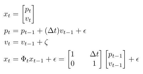
Equation 3

We are assuming that the noise is normally distributed, although the distribution’s parameters may not be the same for both state variables [2]. Let’s also assume that I can only measure my car’s position, so I can write that as [2]:

Equation 4

Where M in this case is a measurement vector [2]. Now that I have set up my problem, I am going to explain pictorially what my Kalman filter is going to do to track my car using Figure 1.

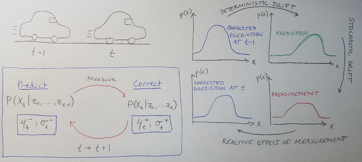
Figure 1 - Source [2]

At time t, I have some prior of the state at the previous time step (if this is the first time step, then the prior is my initial guess; if this is some subsequent time step, then the prior is the corrected prediction from the previous time step) [2]. This prior is the blue Gaussian curve, labeled “corrected prediction at t-1”. I then make a prediction of what I think my state is at the current time step (the green Gaussian curve) [2]. The prediction applies a deterministic drift to the corrected prediction [2]. We say it is deterministic because we know where we are going at the next time step, because we have a model of the dynamics [2]. This prediction shifts my Gaussian because the state is moving - hence the “drift” [2]. I can describe this prediction Gaussian using the mean, mu-minus, and the variance, sigma-minus, as shown in the blue box on the left of Figure 1 [2]. The minus signs indicate that this is the predicted distribution at the moment before the measurement is taken [2].

Remember that I also added noise to my dynamics model? We see the effect of that on the red curve in Figure 1 [2]. The curve has widened because the noise in the dynamics model has added to the variance of the distribution [2]. In effect, I am less sure about where the car is now that I have made a new prediction, because my model has some noise in it [2]. We call this the stochastic drift [2]. To deal with this stochastic drift, I take a measurement of my car’s current position so that I can increase my certainty about my car’s current state [2]. The “reactive effect of the measurement” is that we tighten the distribution - you can see that the blue curve for the “corrected prediction at time t” is narrower than the distribution shown in red [2]. We can describe this new distribution with the parameters mu-plus and sigma-plus, because they describe the distribution after the measurement was made [2].

This essentially describes the iterative process of the Kalman filter - we shift the distribution, expand it (because our model has noise), measure the system, correct the parameters and shrink the distribution [2]. Now let’s apply some math to this process.

Mathematics Behind the Kalman Filter

Let’s go through the math of making the prediction and correction using Gaussians. We’re going to follow the same logic we used in our previous post about the math underpinning generic filters, only this time we are going to focus on manipulating the mean and variance of the Gaussian distributions. Let’s begin with the prediction.

Prediction

Recall that we defined our state to be a normally distributed probability that x has a certain value at time t-1 [2]. This means that when we are predicting what the value of x will be at time t, that prediction will also be a normal distribution - this is one of the fundamental assumptions of the Kalman filter [2]. We can write this prediction distribution as follows [2]:

Equation 5

We can update the mean and variance of this distribution by applying the state transition matrix, phi, which acts as a scaling term [2]:

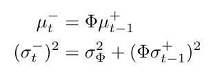
Equation 6

Notice that the variance for the prediction distribution has two terms in it. The first term is the standard amount of variance for the state, per the definition we gave in Equation 1 [2]. The second term adds an additional amount of variance, which is the variance from the measurement taken at the previous time step, scaled by the state transition matrix [2]. Why does this make sense? Recall Figure 1, where we noticed that when we make a prediction, we apply some deterministic drift - that’s the state transition matrix shifting the mean of the Gaussian - and we also apply some stochastic drift [2]. The stochastic drift appears because when we make a prediction, we are now less sure about where the state could be at time t, than we were at the end of time step t-1, when we had measurement data to improve our confidence [2]. We’ll see in a minute that our confidence for the state at time t is going to improve once we take a measurement and correct this prediction [2].

Correction

Just as we saw with the prediction, our corrected probability for the state x at time t given all the measurements z up to and including time t will be a normal distribution [2]. We can write it as follows [2]:

Equation 7

But this time the updates to the mean and variance are more complicated, because they are now going to include both the prediction’s mean and variance, and the measurement’s mean and variance [2]. Let’s see what that looks like [2]:

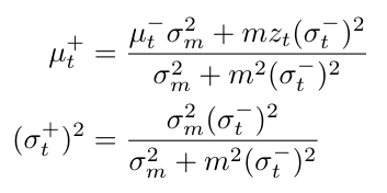
Equation 8

Remember that m is just the measurement matrix. But what is going on in these equations? Let’s consider the mean update as an example, by dividing it through by m-squared [2]:

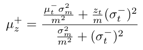
Equation 9

The first term in the numerator has mu-minus, which is our prediction’s best guess of x at time t [2]. The coefficient of mu-minus, sigma-m-squared/m-squared, is the variance of x computed from the measurement only [2]. The second term in the numerator, z/m, is just the measurement guess of x (see Equation 4) [2]. And it’s coefficient is the variance of the prediction of x at time t [2]. In short, the entire expression for mu-plus is a weighted average of the prediction and the measurement, where the weights are the variances of the prediction and measurement [2]. You can see that the denominator contains the sum of the weights, or the sum of the variances of the prediction and the measurement [2].

The idea that the Kalman filter is merging the prediction and measurement information as a weighted average should make sense intuitively [2]. The beauty of the filter is that it combines disparate pieces of information to make predictions about a hidden state, and a weighted average is a good way to do this [2]. The weighted average allows us to give each piece of information a weight that corresponds to how much we believe that that piece of information is correct [2]. For example, if your prediction had no variance - in other words, if you were completely certain about your prediction - then the corrected mean would just be equal to the prediction’s mean [2]. That makes sense intuitively, right? If you completely believe your prediction, then you should just use it without considering the measurement at all.

Wrapping Up the Kalman Filter

So we’ve seen here some of the mathematical principles behind the Kalman filter. Obviously there is more to learn before we can implement them in practice, but we know enough now to see when we would want to use a Kalman filter and when we might look for a different solution. Kalman filters are useful in situations where you need a compact, efficient algorithm that can make simple updates quickly [2]. This is why controls engineers like to use them in applications where computing power is limited. However, a Kalman filter forces you to look at everything in the world as a Gaussian, which may not always be true in practice [2]. It also only allows you to make one hypothesis about where your state is at a time (your hypothesis is the mean of your prediction/correction) [2]. And thirdly, the Kalman filter requires the dynamics model to be linear (although if you use an Extended Kalman filter, you can work with nonlinear models by simply linearizing them about the operating point) [2]. To deal with some of these drawbacks, engineers developed the particle filter as an alternative, which we will see in more detail in my next post.

Footnotes:

*I just wanted to define the term “recursive” here because every time I read it I feel uncertain that I really know what it means. In the context of computer science, a function is recursive if it solves simpler, smaller versions of itself [3]. In mathematics, a recursive definition defines the elements in a set by describing them using other elements in the same set [4]. For instance, fractals are recursive. Here’s a sample function that calculates a factorial recursively [3]:

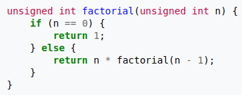
Figure 2 - Source [3]

References:

[1] Bobick, A. “Lesson 43: 7B-L1 Tracking as inference.” Introduction to Computer Vision. Udacity. https://classroom.udacity.com/courses/ud810/lessons/3271928538/concepts/32865685440923 Visited 13 May 2020.

[2] Bobick, A. “Lesson 44: 7B-L2 The Kalman filter.” Introduction to Computer Vision. Udacity. https://classroom.udacity.com/courses/ud810/lessons/3325568562/concepts/33096786070923 Visited 13 May 2020.

[3] Wikipedia. “Recursion.” https://en.wikipedia.org/wiki/Recursion Visited 14 May 2020.

[4] Wikipedia. “Recursive definition.” https://en.wikipedia.org/wiki/Recursive_definition Visited 14 May 2020.