We are back again to revisit another piece of the MolGAN paper and this time we are looking at how they trained their GAN to generate molecules that satisfied particular design criteria [1]. If you recall from the overview of the MolGAN work, they designed a GAN that could generate novel molecules which met some design criteria, like being water soluble or druglike [1]. In order to train the GAN to meet these criteria, De Cao and Kipf used tools from reinforcement learning to optimize their generator [1]. Specifically, they used a policy gradient called Deep Deterministic Policy Gradient (DDPG) [1]. It has been a long time since I have read research related to reinforcement learning, so this post is going to cover some of the basics of reinforcement learning (RL) and introduce the role that policy gradients have in RL. We will introduce algorithms that solve for the policy gradient, such as REINFORCE. In a follow-on post, we will dig into DDPG itself and explain how it works in the context of MolGAN.

Basic and Relevant Ideas in RL

The RL Paradigm

We have previously seen that the paradigm for RL centers around an agent who can take actions in an environment. Every action moves the agent from one state to the next. The probability distribution that defines what state the agent will reach on the next time step is called a transition probability [2]. After every action, the agent receives some reward. In general, the goal in reinforcement learning is to learn a policy (i.e. a way of choosing actions) that optimizes the total rewards that the agent earns [2].

While most of RL is centered around maximizing rewards, it can be divided into two sub-categories [2]. These sub-categories are defined by whether or not we have a model for our situation [2]. The model defines the transition probability and the reward function of the agent [2]. If we do have a model, then we can do model-based RL and we can make a plan given a complete set of information, using techniques like dynamic programming [2]. But if we do not know the model, then we can either try to do model-free RL where we just ignore the fact that we don’t know the model, or we try to explicitly learn the model as part of the process of solving the problem [2].

In the MolGAN paper, we are in a situation where we do not know the model [1]. The policy is the generator itself, and instead of having a state as an input to the policy, the input is a random sample, z [1]. The output of the policy is a graph - the graph is considered an action [1].

Okay, so we have agents that take actions, their states are updated at every time step, and they also receive a reward after every action. But in addition to the reward function, which gives us instantaneous feedback about every action that our agent takes, we also have a value function, which gives us feedback about the long-term success of our actions [2]. The value function is crucial to helping us figure out the optimal policy, because the value function tells us the expected future rewards we will get given that we are in some current state and we are following some policy [2]. The value function is basically giving us a prediction of the total reward we will have at the final state, given where we are now and assuming that we follow a known policy. We use the value function to tell us how good a state is [2].

The take-away message for this section is: To fulfill the reinforcement learning objective of maximizing total reward, we must learn the policy and the value function [2].

Definitions of the Value Function and the Policy

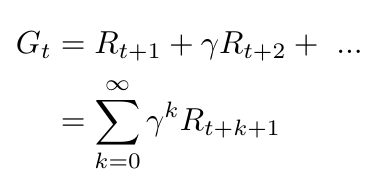
We have seen that our objective in reinforcement learning is to learn the value function and the policy that maximize our total reward. Let’s start by looking at the value function in more detail. We can define the value function as predicting the future reward, or return [2]. We can write an expression for the return by adding up the rewards multiplied by the discount factor [2]:

Equation 1

In reinforcement learning, we will often train an agent by playing out an episode/trial/trajectory, where we examine the situation as a series of sequential time steps [2]. At every time step, the agent performs an action and receives a reward, and in the process it learns about its environment , which helps the agent to also learn a value function and an optimal policy [2]. In MolGAN, the authors did not have episodes because the state-action pair (i.e. the input z, output graph pair) occurred in a single time step [1].

Now let’s consider the policy of the agent. There are two ways to train the agent: (1) on-policy approaches use the deterministic outputs from some target policy in order to train the agent, while (2) off-policy strategies will train the agent on a distribution of transitions (or, for a longer time series, an entire episode) produced by different policies, not necessarily the target policy [2].

Policies can be either deterministic or stochastic, as shown in Equation 2 [2].

Equation 2

In the MolGAN paper, De Cao and Kipf explain that they attempted to use both kinds of policies to model graph generation [1]. I find that interesting because the policy, as we mentioned earlier, is the generator, which I suppose you could consider as stochastic or deterministic. Especially at the beginning of training, the generator would be stochastic as the neural network’s weights would not have been updated yet. Conversely, as the generator learned to output realistic graphs, one could consider the generator to be a more deterministic function. Maybe that explains why De Cao and Kipf could attempt to train the policy using methods that considered the policy to be either deterministic or stochastic.

At any rate, De Cao and Kipf began by training the generator using REINFORCE on a stochastic policy [1]. They explained that the result of this approach was poor convergence because the graph generation process was modeled as a series of discrete actions, but there were so many possible actions that it was difficult to explore that space [1]. They then turned to DDPG and considered the generator as a deterministic policy. We will describe both methods in more detail below.

Some Additional Value Function Definitions

We defined the value function in Equation 1 above. I want to take a moment to define a couple of terms related to the value function that will come in useful later. First, we have the state value of a state: this is the expected return (i.e. value) for this state at some time, t [2]:

Equation 3

Next, we can calculate the action value of a state-action pair [2]. Note that the action value is also called the Q-value, where Q stands for “quality” [2]:

Equation 4

If we are following some target policy, pi, we can also calculate the state value as the sum of the Q-values of every action that the policy could take [2]:

Equation 5

Finally, the action advantage function tells us the benefit of taking a particular action, and is computed as follows [2]:

Equation 6

Now before we move on to discuss policy gradients, I just want to mathematically define the optimal value and policy that we are trying to obtain in this reinforcement learning paradigm. Specifically, we can say that the optimal value function will generate the maximum return possible [2]:

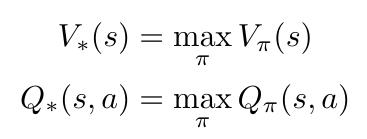
Equation 7

Similarly, the optimal policy is the policy that allows the value function to provide the maximum return [2]:

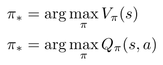
Equation 8

In this section, we presented the fundamental paradigm of reinforcement learning, and learned about the value function and policy that we want to optimize to maximize our total reward. In the next section we are going to discuss methods that we can use to find the optimal policy and the optimal value function.

Policy Gradients

In this section we are going to focus on one class of solutions that solve the reinforcement learning problem of finding the optimal value function and optimal policy. This set of solutions is called policy gradient methods, and is used to learn the policy directly, without learning state and action values first [2].

The reason why we are going to focus on policy gradient methods is that they work well in continuous space, where there are an infinite number of actions that we can take [3]. Let’s think about this in the context of MolGAN: the policy (i.e. the generator) can take an infinite number of actions (i.e. generate an infinite number of graphs). Value-based approaches do not scale well to infinite numbers of actions - we say that they suffer from the Curse of Dimensionality [3].

We can represent our policy as a function parameterized by some value theta, as follows [2]:

Equation 9

We can define our objective function with respect to this parameterized policy function, and we can try to optimize theta to maximize the objective function [3]. First, let’s write the objective function [3]:

Equation 10

Notice that we can see how the value function was expanded by looking back at Equation 5. Also, there is an interesting term in the objective function, d, which is the stationary distribution of the Markov chain for the policy [3]. We have talked about Markov processes before (the key thing to remember is they do not depend on past events), but what is a stationary distribution over a Markov chain?

First, let’s clarify that a Markov chain can be thought of as a discretized version of a Markov process [4]. Second, Lilian Weng tells us to imagine moving along a Markov chain, and to realize that eventually the probability that we will reach a certain state becomes constant [3]. This is called the stationary probability, d [3]. Put another way, the stationary distribution theorem states that if we were following a random walk over a graph, the probability that we would arrive at a certain node (i.e. a certain state) is independent of where we started on the graph [5].

Okay, so now we have defined our policy as some function parameterized by theta, and we have an objective function that we can use to find optimal values of theta that, in turn, optimize our policy and our total return. How, then, do we optimize the objective function, J?

The Policy Gradient Theorem

Spoiler alert: we are going to use gradient ascent to find the value of theta that optimizes the objective function, J [3]. We are very familiar with gradient ascent/descent so in principal this approach is not difficult…but we will see in a minute that this is actually rather difficult. Specifically, it is difficult to actually compute the gradient of the objective function [3]. The gradient of J depends on both the actions (as determined by the policy, pi) and on the stationary distribution, d, which also, indirectly, depends on the policy [3]. It is going to be really difficult for us to figure out how the stationary distribution is affected by changes in the policy [3]. That’s bad news because we are going to be updating the policy as we work to optimize theta [3]. So what do we do?

We can use the policy gradient theorem to rewrite the objective function so that we do not need to find the derivative of the stationary distribution [3]. This new form is going to be much easier to calculate. Unfortunately, I am not going to go through the full proof of why this new form is valid, but Lilian Weng gives an amazing presentation of the proof from Sutton and Barto here [3]. I’ll skip to the end and tell you that we can write the gradient of the objective function as follows [3]:

Equation 11

Cool! Now we have an expression for the gradient of the objective function that we can use to optimize the policy. But there is one more step that I am going to take before we move on to talk about REINFORCE and DDPG; we can rewrite Equation 11 as an expectation.

As Sutton and Barto explain in [6], in this approach,we are going to take samples of the gradient and we will show that the expectation of these samples is proportional to the actual gradient [6]. Notice that Equation 11 is proportional to the gradient, matching this explanation.

Now, Weng provides a little bit of explanation as to how we arrive at Equation 12, but to be honest with you I am not sure exactly why the derivation is valid [3]. Specifically, I am not sure where the sum of the stationary distributions over all states went. Returning to Sutton and Barto, they say that the expression on the right hand side of Equation 12 contains “a sum over states weighted by how often the states occur under the target policy, [pi]; if [pi] is followed, then states will be encountered in these proportions” [6]. I am guessing that this means that we don’t have to worry about the stationary distribution because as long as we are following the target policy, the stationary distribution will naturally appear in our samples anyway. Please let me know if you have a better explanation!

Anyway, let’s take a look at Equation 12 [3]:

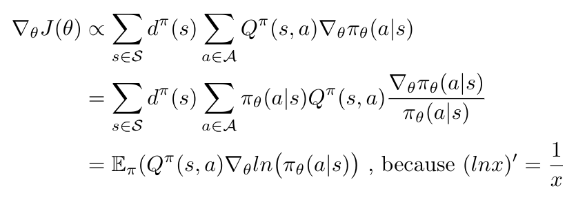
Equation 12

This expression for the policy gradient has no bias but it does have high variance [3]. The algorithms that we are going to study next (REINFORCE and DDPG) are designed to reduce this variance, while keeping the bias at zero [3].

REINFORCE

Let’s start with the REINFORCE algorithm, because it is one of the first policy gradient algorithms, developed by Ronald Williams in the late 1980s - early 1990s [7]. REINFORCE is also called a Monte Carlo*1 policy gradient, which means that it computes an estimate of the total return given a lot of episode samples [3]. This estimate of the total return is used to update theta, the parameter for the policy function, f [3].

REINFORCE relies on the fact that the expectation that we compute over a large number of sampled gradients for the objective function is equal to the actual gradient of the objective function [3]. Recall in Equation 12 that the gradient is dependent on the Q-values of the state-action pairs; we can replace the Q-values with the return, G-t, as shown in Equation 4 [3]. Let’s see how that works [3]:

Equation 13

Okay, so now we have a way to easily compute the gradient of the objective function for a given policy, using the estimated return, G-t [3]. REINFORCE works as shown in the algorithm below [3, 9]:

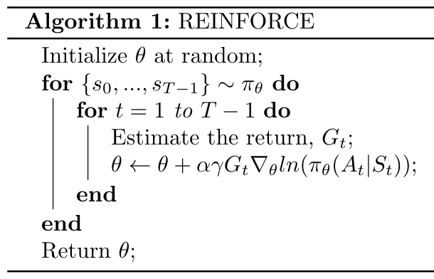
Algorithm 1

The method shown in Algorithm 1 is essentially using stochastic gradient descent over a large number of trajectories to optimize theta [3, 9].

One last note before we move on to DDPG: there is a variation on REINFORCE that subtracts some baseline value from G-t [3]. This variation reduces the variance of the gradient estimate without affecting the zero bias, as we mentioned we wanted to do in our discussion about the policy gradient theorem [3]. For example, we might use the action advantage function, instead of the return [3].

Conclusion

We have now learned the fundamentals of reinforcement learning. We have seen that our objective in RL is to optimize the value function and the policy so that we can maximize our total return. We have introduced policy gradient methods that help us to find the optimal policy, and we have seen one specific method, REINFORCE, in more detail. In the next post, I am going to explore the actual algorithm used by MolGAN, which is called Deep Deterministic Policy Gradients (DDPG).

Footnotes:

*1 Monte Carlo methods is a group of approaches that all use random sampling in order to compute results [8]. A simple example I learned early in grad school was how to compute the value of pi: you generate a circle with radius 1 inside a square, and randomly sample points inside and outside the circle [8]. The ratio of the points that are inside the circle compared to those outside the circle gives you the value of pi with great accuracy if you are using a large number of points [8].

References:

[1] N. De Cao and T. Kipf, “MolGAN: An implicit generative model for small molecular graphs,” arXiv Prepr. arXiv 1805.11973, May 2018.

[2] Weng, L. “A (Long) Peek into Reinforcement Learning.” Lil’Log. 19 Feb 2018. https://lilianweng.github.io/lil-log/2018/02/19/a-long-peek-into-reinforcement-learning.html Visited 04 Aug 2020.

[3] Weng, L. “Policy Gradient Algorithms.” Lil-Log. 8 Apr 2018. https://lilianweng.github.io/lil-log/2018/04/08/policy-gradient-algorithms.html Visited 04 Aug 2020.

[4] “Markov chain.” Wikipedia. https://en.wikipedia.org/wiki/Markov_chain Visited 04 Aug 2020.

[5] Kun, J. “Markov Chain Monte Carlo Without all the Bullshit.” Math Intersects Programming. 6 Apr 2015. https://jeremykun.com/2015/04/06/markov-chain-monte-carlo-without-all-the-bullshit/ Visited 04 Aug 2020.

[6] Sutton, R and Barto, A. “Reinforcement Learning: An Introduction.” 2nd ed, in progress. 5 Nov 2017. The MIT Press, Cambridge, Massachusetts. http://incompleteideas.net/book/bookdraft2017nov5.pdf Visited 04 Aug 2020.

[7] Williams, R.J. Simple statistical gradient-following algorithms for connectionist reinforcement learning. Mach Learn 8, 229–256 (1992). https://doi.org/10.1007/BF00992696

[8] “Monte Carlo method.” Wikipedia. https://en.wikipedia.org/wiki/Monte_Carlo_method Visited 05 Aug 2020.

[9] Yoon, C. “Deriving Policy Gradients and Implementing REINFORCE.” Medium. 29 Dec 2018. https://medium.com/@thechrisyoon/deriving-policy-gradients-and-implementing-reinforce-f887949bd63 Visited 05 Aug 2020.