Okay, so we have now learned how graph convolution works, and we are ready to apply it to a relational graph convolutional network (R-GCN). In this post we will look at another paper by Prof. Welling’s group, this time applying the concept of graph convolution to R-GCNs [1]. This paper uses R-GCNs to complete missing information in knowledge graphs [1]. Specifically, the R-GCN is used to predict what the missing nodes are [1]. The R-GCN is a form of encoder which converts a graph input to some latent space, that can then be used to predict the missing information in the knowledge graph [1]. In this post we will build up the theoretical understanding for how this R-GCN works, and in a subsequent post we will then place the R-GCN in the context of the MolGAN architecture [2].

R-GCN’s Graph Propagation Function

First, I just want to clarify where the term “relational” comes from in this context. Schlichtkrull et al. define “relational” as referring to multigraphs* that have directed and labeled edges [1]. They define their propagation function as follows [1]:

Equation 1

Here N is the set of indices of the neighbors of node i that have relation r, which comes from the set of relations, R [1]. The coefficient c is a normalization constant that Schlichtkrull et al. say can either be treated as a learned parameter or a constant set in advance (for example c could be the absolute value of the set of nodes, N) [1]. Let’s understand where this expression comes from, given what we know about graph convolution from [3].

In [3], we learned that the output of a graph convolution applied to a layer can be written as follows:

Equation 2

Equation 2 is essentially the same as Equation 1 in the special case where all the relations between all the nodes are the same (i.e. they are not relational, they are undirected and unlabeled). Why is this true? Because the multiplication AHW is adding up the feature vectors for all the nodes that are connected to each other, just as we are summing over all nodes in Equation 1. The difference is that Equation 1 is also summing nodes up according to their relationship - all nodes that have the same relationship are added together. The second term in Equation 1 also has an equivalent term in Equation 2. Recall that A-hat in Equation 2 involves A~, which is just the adjacency matrix with a self-loop added to it [1]. In both Equation 1 and Equation 2, we include a self-loop or a self-connection so that when we forward propagate information from one layer to the next, we include information from the node itself to the output for the next layer. I argue that Equation 1 and Equation 2 would be the same if the set of relations contained only one relation.

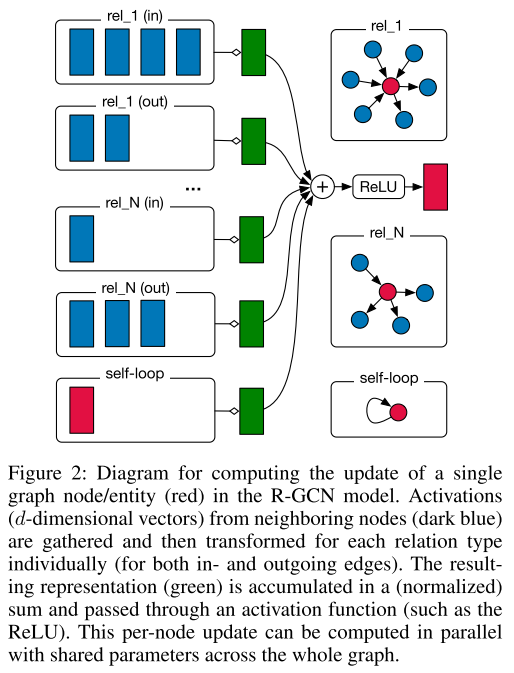
Schlichtkrull et al. present Equation 2 graphically, as shown in Figure 1 [1].

Figure 1 - Source: [1]

Loss Function

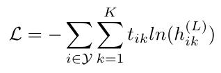
Now we understand how the relationships between nodes in a graph are accounted for in R-GCN. The other piece of this puzzle is understanding the loss function that we will use to optimize the neural network. Schlichtkrull et al. only compute the loss on the labeled nodes, and they do so as follows [1]:

Equation 3

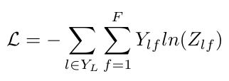
Here Y is the set of indices that refer to labeled nodes. The values t are the “ground truth” labels for the i-th node. This expression matches the form we saw previously in Equation 15, and repeated below [3]:

Equation 4

The only difference between Equations 3 and 4 is that Equation 3 directly compares the labels of the nodes instead of Equation 4, which compares their indices.

We have now presented how we can extend the idea of graph convolutional networks to accommodate graphs that are “relational” (i.e. that have directed and labeled edges). This was important to learn because MolGAN needs to be able to work with relational graphs, since molecules have labeled edges representing different bond types. In the next post, we will return to the MolGAN paper and present how the R-GCN framework is used to build the discriminator and the reward function.

Footnotes:

*Multigraphs are graphs which are permitted to have multiple edges connecting the same pair of nodes [4].

References:

[1] M. Schlichtkrull, T. N. Kipf, P. Bloem, R. van den Berg, I. Titov, and M. Welling, “Modeling Relational Data with Graph Convolutional Networks,” in Lecture Notes in Computer Science (including subseries Lecture Notes in Artificial Intelligence and Lecture Notes in Bioinformatics), 2018, vol. 10843 LNCS, pp. 593–607.
[2] N. De Cao and T. Kipf, “MolGAN: An implicit generative model for small molecular graphs,” arXiv Prepr. arXiv 1805.11973, May 2018.

[3] T. N. Kipf and M. Welling, “Semi-Supervised Classification with Graph Convolutional Networks,” 5th Int. Conf. Learn. Represent. ICLR 2017 - Conf. Track Proc., Sep. 2016.

[4] “Multigraph.” Wikipedia. https://en.wikipedia.org/wiki/Multigraph Visited 31 Jul 2020.