Today I am going to try to tackle a very impressive (and very dense) paper that was recently published by Veerapaneni et al., a group of researchers at UC Berkeley, Stanford and MIT [1]. Their paper explains how they taught a computer to learn to identify objects in an image, model them as a graph, learn something about their dynamics from videos and then perform manipulation tasks without prior training [1]. It looks like it could be a huge step forward in teaching a computer to reason like a human about its environment (I think it has been out for about 2 weeks as of this post so we should probably wait for the experts to tell us if it’s truly as impactful as I think it is). This paper builds on the ideas about graph networks we previously discussed, and I was particularly interested in how the authors taught a computer to construct a graph network on its own. I am going to try to summarize the major contributions of this paper, and it may take a couple of posts to really capture everything, so please hang on to your hats and get ready to read!

30,000 Foot View of the OP3 Learner

Let’s start by talking about what this paper does on a very high level. The authors say that their ultimate goal is to provide evidence that there is an advantage to modeling a scene in terms of entities and their interactions, especially when you want to complete tasks in an environment that you have not seen before [1]. The authors are drawing on ideas from a paper by Battaglia et al. which argues that the best way to teach an AI to think like a human is to teach it to learn how objects interact [2]. These building blocks of understanding can be combined and used to make inferences about scenes and environments that we have not seen before [2]. For instance, if I know how tennis balls behave in Earth’s gravity, then I can pretty easily imagine what it would look like if I dropped a bucket of tennis balls on the floor, even though I have never seen that happen in real life before.

Veerapaneni et al. present a novel approach to learning about environments using entity abstraction, which they call the object-centric perception, prediction and planning (OP3) learner [1]. (I’ll talk more about entity abstraction below.) OP3 can be classified as a model-based reinforcement learner, because it uses a model of the system in its operation [1]. It is a reinforcement learning approach because, instead of being trained with labeled data or learning to categorize data, it is trying to balance the benefits of exploring and exploiting its environment to maximize a reward [1, 3].

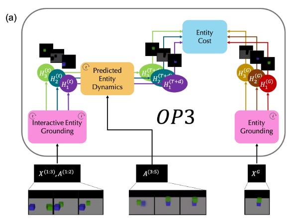
The OP3 approach is summarized in Figure 1. OP3 takes as input a series of images, and then uses a process called “Interactive Entity Grounding” to represent the objects in the image as entities in a graph network [1]. It then learns a dynamics model from observing sequences of images of the objects interacting [1]. Once the algorithm has learned the entity grounding and the dynamics model, it receives a picture of the goal environment [1]. OP3 takes this image and matches the objects in the picture to the entities it has learned and identified, then it computes the difference between the objects’ current positions and their desired goal positions [1]. OP3 plans a series of actions to minimize the cost as quickly as possible to complete the task [1]. As it is planning, the algorithm is capable of making predictions about how the actions will affect the objects in the scene [1]. This is how the algorithm perceives the objects in a scene, makes predictions about them and plans to complete some desired task [1].

Figure 1 - Source: Figure 1(a) in [1]

Let’s talk about what entity abstraction is and see how Veerapaneni et al. use this principle to set up their problem definition.

Entity Abstraction

Veerapaneni et al. say that they use entity abstraction to represent the latent state (i.e. the hidden state of the system) as local entities with their own states [1]. In other words, everything that OP3 does is performed on a group of entities, not on some global representation of the entire system [1]. The authors say that they “enforce the entity abstraction” many times throughout the construction of their learner [1]. Let’s see how they do this by setting up the problem and the different components of the learner.

First, we assume that we are modelling a physical system, which is described as x*, and this system contains some number, K, of objects, h* [1]. Notice that x* and h* are the ground truth, the actual system and its objects, and we cannot observe them directly [1]. The fact that we cannot directly measure our system and the actual objects makes this system partially observable [1]. In fact, we can say that we are setting up a partially observable Markov decision process (POMDP) because we are also going to model our learner as a Markov process* [1,4,5]. We define the observations of the scene x* as X, and the actions of the agent are A [1]. Our latent random variables are H, which represent the state of the objects, h*; there are K instances of H, one for each object [1]. This is where the “entity” in “entity abstraction” comes from: the authors make the distinction that h* represents objects, but H represents entities [1]. The entities are part of the model of the physical world; the objects are part of the actual physical world [1].

The OP3 learner’s powerful ability to perceive and model a POMDP given observations, entities and actions can be summarized in Equation 1 [1]. Equation 1 describes the probability of obtaining some number, T (corresponding to a number of time steps), of observations and entity states, given that we take some actions, a [1]:

Equation 1 - Source: Equation 1 in [1]

Okay, that is kind of a hot mess of an equation, so let’s break it down a little. The final term, the product of T probabilities P(X given H), is the observation model computed over all the time steps, t = T [1]. The middle term, the product of the probabilities P(H at t given H for t-1, a for t-1), is the dynamics model over all time steps [1]. But why does the equation take this form? The left hand side is the joint probability that we would get both the observations and entities from the initial time to time T [1,6]. We know from our discussion on MLE vs MAP that we can rewrite the joint probability P(A,B) = P(A)P(B) which is what we have done in Equation 1 [1,6]. Moreover, notice two other things: for the observation model, we assume that the observation X at time t only depends on the state of the objects H at time t [1]. And the dynamics model assumes that the state of the objects only depends on the state of the objects at the previous time step, t-1, and on the action just taken at t-1 [1]. We can make these assumptions because we have a Markovian process which assumes that our state at time t only ever depends on the state and actions from the immediately previous time step, t-1. You can read more about this in my discussion on filtering.

Now that we have seen how OP3 perceives and models a series of observations and entity states from a sequence of actions, we need to be able to predict what will happen in the future. In other words, we need to be able to compute Equation 2 [1]:

Equation 2 - Source [1]

The authors call this the posterior predictive distribution of observations, which means that it is a probability distribution about some statistical process (our POMDP system) that is based both on prior knowledge of the system model, as well as the likelihood of the observations that we obtain at the current time step [1]. This is where things get really interesting. Do you remember our discussion of a variational autoencoder, and how we used Bayesian variational inference to optimize the VAE’s representation of the latent space? We are going to use this approach again in this paper. In my next post, I will go into detail about how to perform Bayesian variational inference and how it is used in this paper.

Footnotes:

*A partially observable Markov decision process (POMDP) assumes that an agent is making some decisions according to a process, inside some system whose dynamics are Markovian [4]. The agent cannot directly see the underlying state of the system, instead it is computing a probability distribution over a set of possible states using observations that produce an observation model [4]. Mathematically, we define a POMDP to have an agent, A, some states, S, and some observations, Z [5]. The states are updated by some transition, T, and the observations can be modeled using an observation model, O(S,Z) which tells you the probability of getting observations Z if the agent is in state S [5]. The agent can earn rewards based on some reward function, R [5].

References:

[1] R. Veerapaneni et al., “Entity Abstraction in Visual Model-Based Reinforcement Learning,” Oct. 2019. ArXiv ID: 1910.12827 https://arxiv.org/abs/1910.12827

[2] P. W. Battaglia et al., “Relational inductive biases, deep learning, and graph networks,” Jun. 2018. ArXiv ID: 1806.01261. https://arxiv.org/abs/1806.01261

[3] Wikipedia. “Reinforcement learning.” https://en.wikipedia.org/wiki/Reinforcement_learning Visited 20 May 2020.

[4] Wikipedia. “Partially observable Markov decision process.” https://en.wikipedia.org/wiki/Partially_observable_Markov_decision_process Visited 19 May 2020.

[5] Udacity. “POMDPS.” From course “Reinforcement Learning”, video hosted on YouTube. https://www.youtube.com/watch?v=1TRoIuvWNuI&list=PL__ycckD1ec_yNMjDl-Lq4-1ZqHcXqgm7&index=189 Visited 20 May 2020.

[6] Wikipedia. “Joint probability distribution.” https://en.wikipedia.org/wiki/Joint_probability_distribution Visited 20 May 2020.