Today we are going to continue building on ideas from spectral graph theory to define an expression for convolution over a graph. This theory is based on several papers by Prof. Max Welling’s team of researchers at the University of Amsterdam into generating novel graphs using relational graph convolutional networks (R-GCNs) [1, 2] and generative adversarial models (GANs) [3].

In this post, we will begin by understanding how we can use spectral graph theory to convert the representation of a graph from the “node domain” to the Fourier domain [4]. Then we will apply this idea to writing the expression for graph convolution, going into detail to explain how this expression was obtained.

The Graph Fourier Transform

Kipf and Welling tell us that a spectral convolution of a graph is done by multiplying some signal, x, with a filter, g, expressed in the Fourier domain [2]. Huh?

Let’s cover a little more spectral graph theory. It is possible to have a graph Fourier transform - a graph Fourier transform will decompose the Laplacian, L, into eigenvalues and eigenvectors [4]. This is similar to Fourier transforms for scalars because we can think of the eigenvalues as different frequencies (as represented by s in the Fourier domain) [4]. The eigenvectors can be thought of as a graph Fourier basis [4]. Also note that because the Laplacian is symmetric, its eigenvectors specifically form an orthogonal graph Fourier basis [4].

What does the graph Fourier transform look like? Let’s say we have a graph, G = (V, E). We can have a graph signal, f, that maps the nodes of the graph to some real scalar value, like so [4]:

Equation 1

Any graph signal, f, can be projected onto the eigenvectors of the Laplacian of the corresponding graph [4]. If we denote the eigenvalues of the Laplacian as lambda, and the eigenvectors as mu, then we can write the graph Fourier transform as follows [4]:

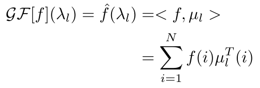
Equation 2

Similarly, the inverse function exists since the eigenvectors of the Laplacian are orthogonal [4]:

Equation 3

That was a lot of detail, but hopefully you can see now that the graph Fourier transform is very similar to the classic Fourier transform, and it allows us to move between the node domain of the graph, f(i), and the graph spectral domain, f(lambda) [4]. In the next section, we will see how we use this transform to write an expression for graph convolution.

Graph Convolution

Let’s return to see how convolution can be written in the Fourier domain according to Kipf and Welling [2]:

Equation 4

We can define U as the matrix of eigenvectors of the normalized graph Laplacian, in other words [2]:

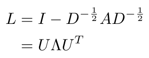
Equation 5

Kipf and Welling also tell us that by multiplying U-transpose with x, we are performing the graph Fourier transform of x [2]. That makes sense because it matches the graph Fourier transform we showed in Equation 2. Also, recall that convolution in the graph node domain (similar to the time domain from the classical control perspective of the Fourier transform) is equal to multiplication in the Fourier domain. That means that g multiplied with Ux is the Fourier domain equivalent operation to convolution in the node domain. Finally, we multiply the result of this convolution with U to perform the inverse graph Fourier transform to return a final value in the graph node domain.*

Okay, so Equation 4 convolves a graph via its Laplacian. We’ve done it! We can do graph convolution! However, Kipf and Welling point out that it is computationally expensive to compute Equation 4 directly [2] and so they suggest that we can approximate the filter, g, with a short expansion in Chebyshev polynomials** [2]:

Equation 6

Now that I have this approximation, I will go through the manipulations that I think Kipf and Welling used to arrive at their final expression for a K-th order approximation of graph convolution (they only gave the final equation in their paper) [2]:

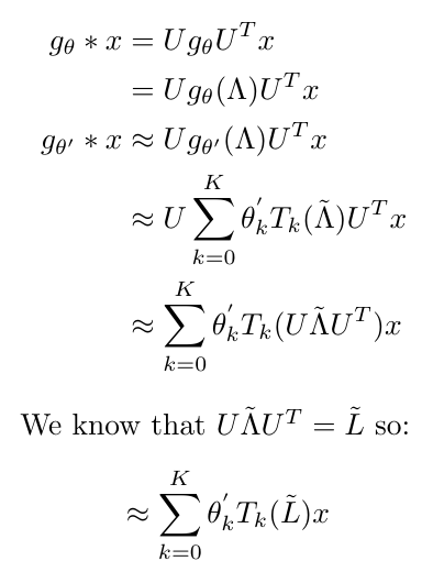
Equation 7

This ultimately results in [2]:

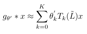
Equation 8

Kipf and Welling tell us that this approximation is a K-th order polynomial with respect to the Laplacian [2]. This means that this expression will convolve nodes that are up to K “hops” away from the node in question [2]. Kipf and Welling argue that this approximation is much easier computationally because the computation time scales linearly with the number of edges in the graph [2].

Now that we have this K-th order approximation, let’s see what a first-order approximation would look like, and how we can use it to write the graph propagation function that we saw last time.

From Graph Convolution Back to the Graph Propagation Function

We are going to look specifically at the first order form of the approximation shown in Equation 8. You might be wondering why we want to use the simple first order form when we could choose a more complex approximation. Great question! Kipf and Welling explain that they chose to use the first-order form because it is a linear function that is easily calculated [2]. More importantly, as you will see in a minute, the first order expression does not actually have any of the Chebyshev polynomial structure, even though we used Chebyshev polynomials to derive it [2]. This is valuable because we want our model to be as general as possible, and if we had an explicit Chebyshev polynomial structure in our function, we might be more likely to overfit our model to the graph in a certain way [2]. If you think back to our discussion of relational inductive biases, including the Chebyshev polynomial structure would be like adding additional inductive bias. It might help, but it is more likely to force our neural networks to think in a way that is too specific and not general enough for all the different kinds of graphs that we are likely to see.

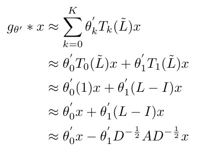
So we have now explained why we will choose to use K = 1 in our approximation of graph convolution. We should also note that we choose the maximum eigenvalue to be 2 in this approach [2]. Kipf and Welling explain that they predicted that the value of the maximum eigenvalue would not really matter, because the neural network weights would adapt to whatever value they chose [2]. Now that we have defined these two parameters, we can write out our first order approximation. I will show you my working out that led me to obtain the equation that Kipf and Welling obtained in their paper [2]:

Equation 9

We say that the theta-prime values are free parameters, and all the parameters describing the filter, g, can be shared over the entire graph [2]. Notice that in its final form, this expression does not show any of the Chebyshev structure that we saw in Equation 6.

Even though this approximation is first order, Kipf and Welling will stack multiple layers of convolution to convolve increasingly larger neighborhoods of the graph [2]. Since they do stack layers, they decided to simplify the convolution function to have only one parameter, theta, to avoid overfitting and reduce computational time, leaving us with the following expression [2]:

Equation 10

Kipf and Welling point out that this function can lead to numerical instabilities and either vanishing or exploding gradients when multiple layers of convolution are stacked on top of each other [2]. They addressed this problem by applying what they call a “renormalization trick” which just re-writes the expression inside parentheses in Equation 10 as follows [2]:

Equation 11

I’m not completely sure why this expression is more numerically stable; it might be because on every layer of convolution, we renormalize the adjacency and degree matrices so that they do not shrink or explode over time.

We are almost there. Now that we have a “renormalized”, first order approximation for graph convolution, we can write an expression for the convolved signal, Z, in terms of the adjacency and degree matrices of the graph, the input signal, X, and the matrix of filter parameters, theta [2]:

Equation 12

Here, Z is a N x F matrix where N is the number of nodes and F is the number of filters [2]. Theta is a matrix of size C x F where C is the number of input channels (i.e. each node will have C features) [2]. This operation now has computational complexity that is linearly proportional to the number of edges x F x C [2]. The AX operation is efficient because we are multiplying a sparse matrix (A) with a dense matrix (X) [2].

Now let’s link Equation 12 back to the graph propagation function from last time. In the last post, we wrote the graph propagation function as follows [2]:

Equation 13

Recall that we said that the output of the graph propagation function for the l-th layer is Z, and the value of H at the 0-th layer is X. We also can replace the matrix of filter parameters, Theta, with the matrix W in Equation 13. Kipf and Welling decided to experiment with their novel GCN using a two-layer implementation, which means that the entire graph propagation function can be written as a single equation as follows [2]:

Equation 14

Note that A-hat is a “pre-processing step” that performs the “renormalization” of the adjacency matrix prior to performing the graph convolution operation [2]. In this implementation, W-0 is a C x H size matrix, and W-1 has dimensions H x F. The softmax activation function on the output layer is applied row-wise.

Do you see how we have now come full circle? We intuitively obtained an expression for the graph propagation step at the beginning, and we have now shown that the graph propagation function is equivalent to a graph convolution operation. Cool, right?

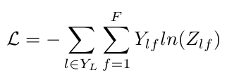
Before we end, I want to just give the expression for the cross-entropy error that the authors used to train this neural network so that it could perform multiclass classification [2]:

Equation 15

The weights, W-0 and W-1, are trained using gradient descent [2]. The matrix Y is the set of indices for labeled nodes [2].

Okay, so in this post we have learned how graph convolution works and how Kipf and Welling applied it using a neural network approach. This is a key insight that we will carry into our next post where we will discuss how this graph convolution function is used to build R-GCNs. In future posts we will then return to the MolGAN paper and understand the role that R-GCNs play inside the MolGAN architecture.

Footnotes:

*I am not sure this interpretation is correct. Let me know if you have a better one.

**I won’t go into detail on Chebyshev polynomials here beyond saying that they are frequently used to approximate other functions [5]. They have a nice property where Chebyshev polynomials have roots that we can use to fit them to polynomial functions, which is why they are so useful for approximations [5].

References:

[1] M. Schlichtkrull, T. N. Kipf, P. Bloem, R. van den Berg, I. Titov, and M. Welling, “Modeling Relational Data with Graph Convolutional Networks,” in Lecture Notes in Computer Science (including subseries Lecture Notes in Artificial Intelligence and Lecture Notes in Bioinformatics), 2018, vol. 10843 LNCS, pp. 593–607.

[2] T. N. Kipf and M. Welling, “Semi-Supervised Classification with Graph Convolutional Networks,” 5th Int. Conf. Learn. Represent. ICLR 2017 - Conf. Track Proc., Sep. 2016.

[3] N. De Cao and T. Kipf, “MolGAN: An implicit generative model for small molecular graphs,” arXiv Prepr. arXiv 1805.11973, May 2018.

[4] “Graph Fourier Transform.” Wikipedia. https://en.wikipedia.org/wiki/Graph_Fourier_Transform Visited 30 Jul 2020.

[5] “Chebyshev polynomials.” Wikipedia. https://en.wikipedia.org/wiki/Chebyshev_polynomials Visited 30 Jul 2020.